Inverse Kinematics on Kuka Arm using ROS and Python

Contents:

Picking and placing objects is something that we as humans take for granted. That's not the case for our mechanical(and electronic) friends. They have to

Calculate an optimal collision-free path from the source to target location.
Perform inverse kinematics to control the joints on your arm.
Pick the object cleanly,without knocking over other objects in your path(well, this one doesn't always go very well for us either).

One of the most challenging projects that I did in my Udacity Robotics Nanodegree program was to control a 6-jointed robot arm to pick and place an object.

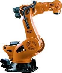
I was given a trajectory that the arm should follow to reach the object, pick up and drop it at a given location. My job was to perform inverse kinematic analysis to calculate the joint positions that will move the gripper along the requested path.

Enter math.

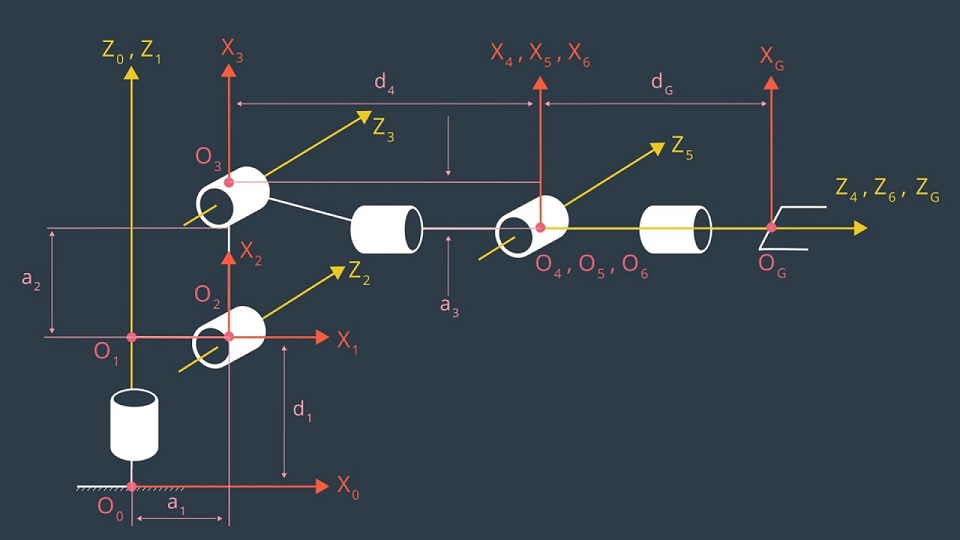
Fig. 1 : Shows the link frames(coordinate systems) choosen according to Modified DH convention discussed next. $O_i$ is the origin for link $i$ frame, and $X_i$, $Z_i$ are the $X$ and $Z$ axis correspondingly, and $Z$ represents the axis of rotation(translation in case of prismatic joints). Since we are using a right handed coordinate system, $Y_i$ can be calculated accordingly.

Here is a diagram of the gripper showing the degrees of freedom that the arm has, along with their reference frames. Computing through these transformations can become complex and tedious really fast. So, we use a convention.

Denavit–Hartenberg Analysis

The Denavit–Hartenberg(DH) convention is a commonly used system for selecting the frames of reference in robotics applications. They are particularly designed to cut out the number of free parameters required to specify the whole system. Here is an illustration,

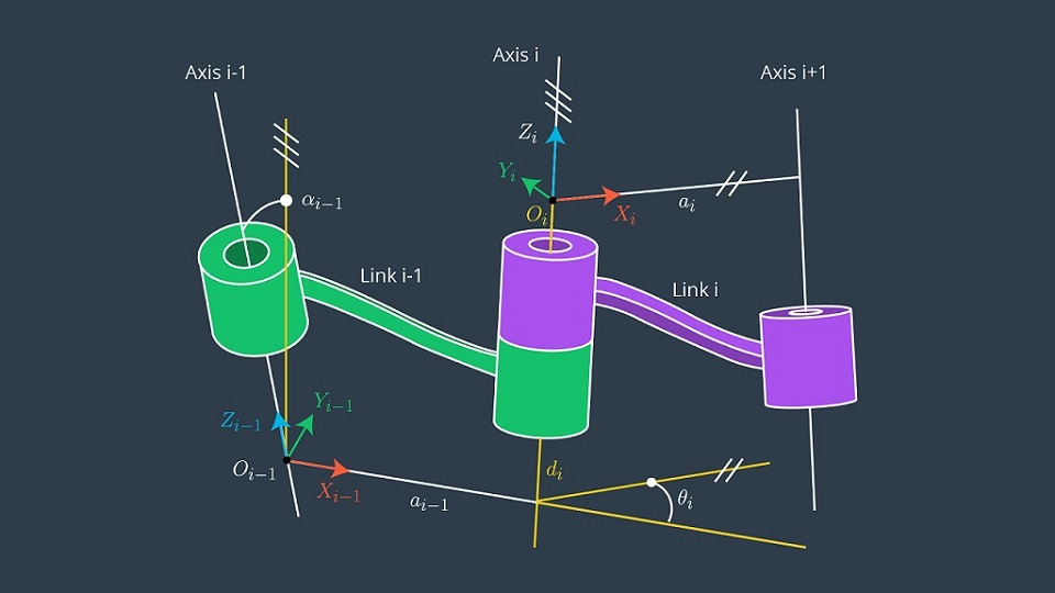Fig. 2 : Modified DH convention axes assignment and parameters.

Here,

$d_i$ : Link offset, distance between $X_{i-1}$ and $X_i$, measured along $Z_{i-1}$, variable in prismatic joints.
$\alpha_{i-1}$ : Angle between $Z_{i-1}$ and $Z_i$, measured along $X_i$.
$a_{i-1}$ : Link length, distance between $Z_{i-1}$ and $Z_i$, measured along $Z_{i-1}$.
$\theta_i$ : Joint angle, Angle between $X_{i-1}$ and $X_i$, measured along $Z_i$, variable in revolute joints.

So, according to this convention, the total transform between links $L_{i-1}$ and $L_i$ can be thought of as a roation by $\alpha_{i-1}$ along $X_{i-1}$, translation by $\alpha_{i-1}$ along $X_{i-1}$, rotation by $\theta_i$ along $Z_i$, and finally translation by $d_i$ along $Z_i$. That is,

$$ T_{i-1}^{i} = R(x{i-1},, \alpha_{i-1}) \cdot T(x_{i-1}, a_{i-1}) \cdot R(z_i, \theta_i) \cdot T(z_i, d_i)$$

Which, when expanded analytically, turns out to be,

$$\begin{eqnarray} T_{i-1}^{i} = \begin{bmatrix} cos(\theta_i) & -sin(\theta_i) & 0 & a_{i-1} \\ sin(\theta_i)cos(\alpha{i-1}) & cos(\theta_i)cos(\alpha{i-1}) & -sin(\alpha{i-1}) & -sin(\alpha{i-1})d_i \\ sin(\theta_i)sin(\alpha{i-1}) & cos(\theta_i)sin(\alpha{i-1}) & cos(\alpha{i-1}) & cos(\alpha{i-1})d_i \\ 0 & 0 & 0 & 1 \end{bmatrix} \end{eqnarray}$$

Now, we can apply this convention to our robotic arm and find out all the required parameters for further analysis. Here are the model specifications and final DH-parameters,

$Link_i$	$\alpha_{i-1}$	$a_{i-1}$	$d_i$	$\theta_i
1	0	0	0.75	q1
2	-pi/2	0.35	0	q2 - pi/2
3	0	1.25	0	q3
4	-p1/2	-0.054	1.50	q4
5	pi/2	0	0	q5
6	-pi/2	0	0	q6
7(G)	0	0	0.303	0

Referring back to the transformation equation (1), transformation between two links can be defined separately, we use sympy for symbolic computation, simplification and substitution.

# Create transformation matrix between two links 
# according to Modified DH convention with given parameters  
def createMatrix(alpha, a, q, d):
    mat =  Matrix([[            cos(q),           -sin(q),           0,             a],
                   [ sin(q)*cos(alpha), cos(q)*cos(alpha), -sin(alpha), -sin(alpha)*d],
                   [ sin(q)*sin(alpha), cos(q)*sin(alpha),  cos(alpha),  cos(alpha)*d],
                   [                 0,                 0,           0,             1]])

    return mat

Also, total homogenous transform between base_link and gripper_link can be computed as,

$$T_0^G = T_0^1*T_1^2*T_2^3*T_3^4*T_4^5*T_5^6*T_6^G$$

And, finally, the same total transform can also be computed given the gripper_link position and orientation w.r.t. base_link.Given,

pg_0  = [px, py, pz] # End effector position.
p_quat = [qx, qy, qz, qw] # End effector orientation as a quaternion.

# R0_g = end-effector(gripper) rotation transformation(4X4)
R0_g = tf.transformations.quaternion_matrix(p_quat)
D0_g = tf.transformations.translation_matrix(pg_0)

T_total = R0_g*D0_g

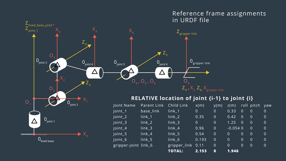
Now, the total transform computed previously, $T_0^G$ is gripper_link transform specified in DH convention(yellow). However, the transform calculated from gripper_link position and orientation is in URDF frame(green). These are shown in the following image,
total-transform-corretion

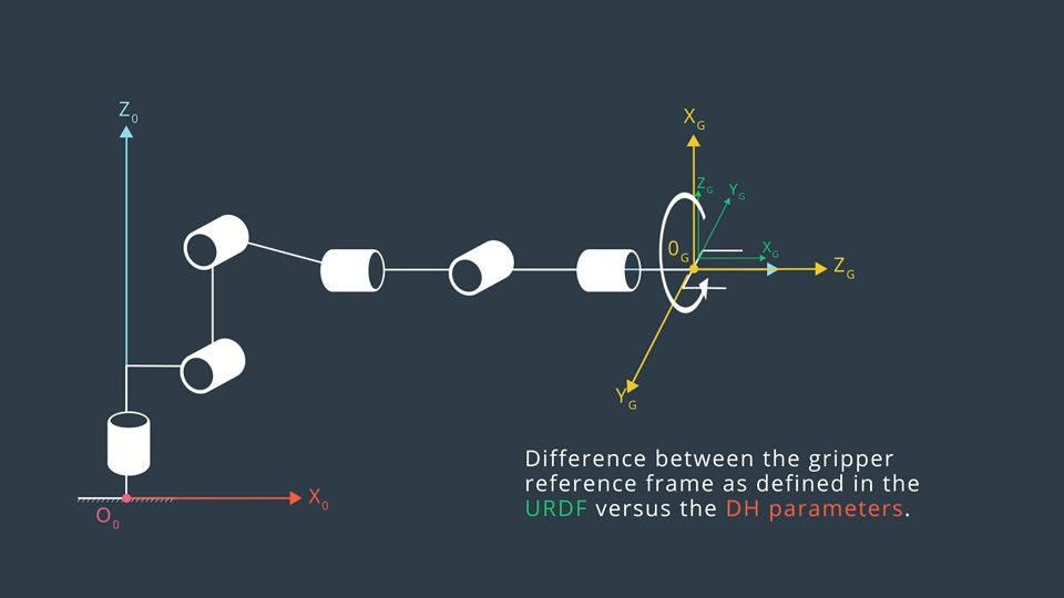
So, we need to correct T0_G transform by rotating by pi along Z, and then by -pi/2 along Y. Thus,
T_total = T0_G*rot_z(pi)*rot_y(-pi/2)

Now the IK part.

The last three joints q4, q5, q6 don't affect the position of Wrist Center(O5), hereby referred to as WC position.(this can be confirmed by running the Forward kinematics demo.) This is very convenient for us in decoupling the IK problem into a position and orientation problem where we can first compute the position of the WC(which gives us the first three joint angles q1, q2, q3) and orientation of the wrist , which gives us the last three joints q4, q5, q6. Detailed explanation follows,

Given End effector position and orientation, we calculate the the wrist center as follows,

# rwc_0 = wrist-center position w.r.t. base_link(O_0)
rwc_0 = pg_0 - (d_g*(R0_g*z_g))

Where,
pg_0 = End effector position received.
p_quat = End effector orientation received as quaternion.
d_g = s[d7] = Displacement of end-effector from wrist center(along z).
R0_g = tf.transformations.quaternion_matrix(p_quat) = End effector rotation matrix.
z_g = rot_z(pi)*rot_y(-pi/2)*([0, 0, 1]) = gripper frame z axis in DH convention.

So, the above equation displaces pg_0 by -d_g in the z direction.

Calculate q1 given WC.

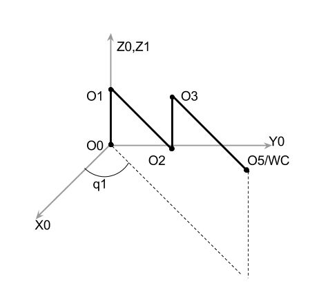
Fig. 7 : Oblique view of the arm, when q1 != 0, all other angles are assumed zero.

From the above image, q1 can be calculated by projecting WC on X0-Y0 plane and calculating angular displacement from X0. i.e.

theta1 = atan2(rwc_0[1], rwc_0[0])

Calculate O2 position according to calculated q1.

# position of O2 w.r.t. base_link in zero configuration, i.e. when q1 = 0
pO2_0 = Matrix([[s[a1]], [0], [s[d1]]])
# Rotate pO2_0 w.r.t. Z by theta1
pO2_0 = rot_z(theta1)* pO2_0

Consider triangle(O2, O3, WC).
Note : Points O0, O1, O2, O3 and O5/WC now lie in the same plane, defined by rotatingplane X0Z0 about Z0.

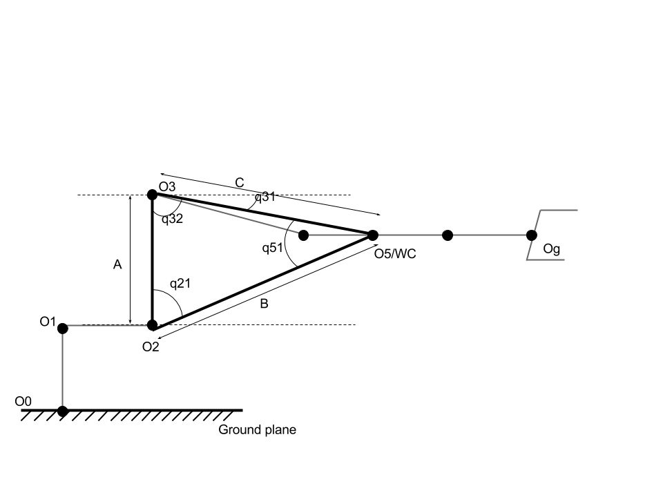
Fig. 8 : Schematic of arm in the plane containing triangle O2, O3, WC. Various angles required dimensions are also shown.

In the figure, position O2, WC are known and length A, B and C are known.

# O2 , WC are known
# O3 = unknown
# Distance between O2 and O3 = a2(in figure 1)
A = s[a2]

# Distance between O2 and O5/WC
pO2towc_0 = rwc_0 - pO2_0
B = pO2towc_0.norm()

# Distance between O3 and O5/WC = (d4^2 + a3^2) in figure 1
C = np.sqrt(s[d4]*s[d4] + s[a3]*s[a3]) 

# Offset angle between the Y3 axis line(O3, O5), -q31 in figure
beta_prime = atan2(s[a3], s[d4])   # From Fig. 1

Now, we can apply Law of cosines in $\Delta(O_2, O_3, O_5)$.

In any triangle(A, B, C)
c.c = a.a + b.b - 2.a.b.cos(alpha),
where alpha = angle(BAC) and `.` represents multiplication

So,

# applying cosine rule `C^2 = A^2 + B^2 -2ABcos(gamma)`
# angle(O3, O2, O5), q21 in figure.
gamma = np.arccos(float((A*A + B*B - C*C)/(2*A*B)))

# angle(O2, O3, O5), q32 in figure 
beta = np.arccos(float((A*A + C*C - B*B)/(2*A*C)))

Find theta2
Next, we need to compute theta2, which can be thought of as the angle between link 2 direction i.e. dir(O2, O3) and X2. Also, dir(O2, O3) can be calculated by rotating dir(O2, WC) by -gamma along Z2.
We can get X2 and Z2 by substituting q1=theta1 (calculated above) in T0_2 and multiplying the result by X(1, 0, 0) and Z(0, 0, 1) respectively. Note : T0_2 = T0_1*T1_2.
So,

# z_2prime is the Z2 axis when q1 = theta1, this does not depend upon q2 
z_2prime = T0_2.subs({q1:theta1}).dot([[0], [0], [1], [0]])

# Rotate pO2towc_0 by gamma along z_2prime
z2_rotation =  tf.transformations.rotation_matrix(-gamma, z_2prime)
# quaternion_about_axis(gamma, z_2prime[0:3])
# tf.transformations.quaternion_from_matrix(z2_rotation)
a_dir = z2_rotation * pO2towc_0
a_dir = a_dir.normalized()

# Compute theta2
X2_prime = self.T0_2.subs({q1:theta1, q2:0}).dot([[1], [0], [0], [0]])
theta2 = np.arccos(float(np.dot(X2_prime, a_dir[0:4]) ))

Find theta3
theta3 is simply the deviation of angle(O2, O3, WC) from pi/2 - q31.i.e.
theta3 = (pi/2 - q31) - q32, But q31 = -beta_prime and q32 = beta, So,

theta3 = (pi/2 + beta_prime) - beta

Now, we need to calculate q4, q5, q6. For this we calculate the rotation matrix R3_6 from our total transform and calculated angles numerically(from end effector position/rotation) and symbolically(from DH parameters). We then compare the two representations to calculate plausible values of the last three joint angles. So,

Symbolically : Just combine the symbollic transformations for individual links from link 3 to 6.

# Extract the rotation component of the matrix,cos that's what we want
>>> R3_6_sym = (T3_4*T4_5*T5_6)[:3,:3] 
[[-s4s6 +c4c5c6,-s4c6 -s6c4c5,-s5c4],
 [         s5c6,        -s5s6,   c5],
 [-s4c5c6 -s6c4, s4s6c5 -c4c6, s4s5]]
# Where, s = sin, c =cos, 4,5,6 = q4,q5,q6
# So that, -s5c6 = -sin(q5)cos(q6)

Numerically :

# Calculate R3_6
R0_g(corrected) = R0_6*R_corr
# Where
R_corr = rot_z(pi)*rot_y(-pi/2)
# So
R0_g = R0_3*R3_6*R_corr
R0_3.T*R0_g*R_corr.T = R3_6

# And,
R0_3 = T0_3[0:3,0:3]   # Extract the rotation matrix
R3_6 = R0_3.transpose()* Matrix(R0_g)*self.R_corr.transpose()

Finally we can evaluate this Matrix numerically by substituting q1, q2 and q3 calculated above

R3_6 = R3_6.subs({q1: theta1, q2:theta2, q3: theta3})

Now, we need to select suitable terms from the matrix to compute q4, q5, q6. We just follow the strategy of selecting the simplest terms to give to atan2 function for a given angle. i.e.
theta4 = atan2(R3_6[2,2], -R3_6[0, 2]), Since,
R3_6[2,2]/-R3_6[0, 2] = sin(q4)sin(q5)/sin(q5)cos(q4) = tan(q4)

theta5 = atan2(sqrt(R3_6[0, 2]*R3_6[0, 2] + R3_6[2, 2]*R3_6[2, 2]), R3_6[1, 2]), Since,
sqrt(R3_6[0, 2]*R3_6[0, 2] + R3_6[2, 2]*R3_6[2, 2]) = sin(q5),
sqrt(R3_6[0, 2]*R3_6[0, 2] + R3_6[2, 2]*R3_6[2, 2])/R3_6[1,2] = sin(q5)/cos(q5) = tan(q5)

And finally, theta6 = atan2(-R3_6[1,1], R3_6[1, 0]), Since,
-R3_6[1,1]/-R3_6[1, 0] = sin(q5)sin(q6)/sin(q5)cos(q6) = tan(q6)

This completes the Inverse Kinematic Analysis of the Kuka arm.

Computing Errors :

Since all these computations are done numerically, they are bound to accumulate error, here is a plot showing the error in positions generated by the results of IK during a sample trajectory.

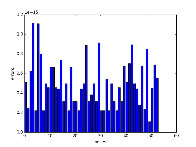
Such low error values show the stability of the computed trajectory using the analysis discussed above.
All of the code and more explanations can be found at my github repository.

Here is badly edited video of the awesome robot in action.

Next Steps

This was a really good learning experience as well as a refresher for me. I got very familiar to the ROS and RViz interface, played with Gazebo and reinforced my knowledge of kinematics. And I got to introduced sympy, which now I absolutely love for its simplicity and power.
That said and done, its time to apply this experience on an actual robotic arm. So stay tuned for that...!!!

Denavit–Hartenberg Analysis

Now the IK part.

Next Steps

Comments