Style Transfer, Part 2

Contents:

Style Transfer

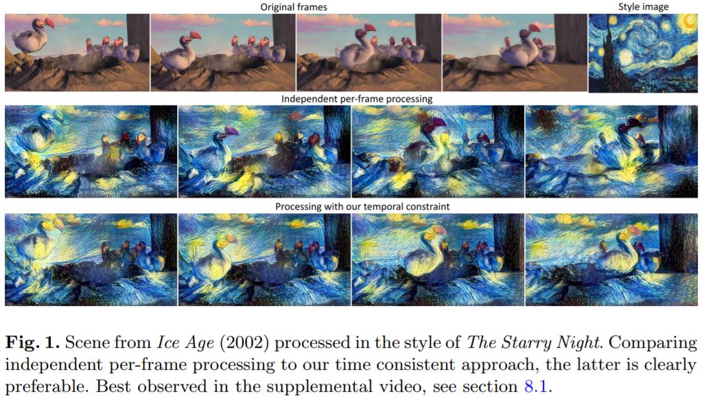
Artistic style transfer for videos

Manuel Ruder, Alexey Dosovitskiy, Thomas Brox : Apr 2016
Source

• The previously discussed techniques have been applied to videos on per frame basis.
• However, processing each frame of the video independently leads to flickering and false discontinuities, since the solution of the style transfer task is not stable.
• To regularize the transfer temporal constraints using optical flow are introduced.
• Notation
  • \(\mathbf p^{(i)}\) is the \(i^{th}\) frame of the original video.
  • \(\mathbf a\) is the style image.
  • \(\mathbf x^{(i)}\) are the stylized frames to be generated.
  • \(\mathbf {x'}^{(i)}\) is the initialization of the style optimization algorithmat frame \(i\).
• Short-term consistency by initialization
  • Most basic way to yield temporal consistency is to initialize the optimization for the frame \(i+1\) with the stylized frame \(i\).
  • Does not perform very well if there are moving objects in the scene, so we use optical flow.
  • \(\mathbf {x'}^{(i+1)}=\omega_i^{i+1}\mathbf x^{(i)}\). Here \(\omega_i^{i+1}\) denotes the function tha warps a given image using the optical flow field that was estimated between \(\mathbf p^{(i)}\) and \(\mathbf p^{(i+1)}\).
  • DeepFlow and EpicFlow, both based on Deep Matching are used for optical flow estimation.
• Temporal consistency loss
  • Let \(\mathbf w = (u,v)\) be the optical flow in forward direction and \(\mathbf {\hat w}=(\hat u, \hat v)\) the flow in backward direction.
  • Then, \(\mathbf {\tilde w}(x,y) = \mathbf{w}((x,y) + \mathbf{\hat{w}}(x,y))\) is the forward flow warped to the second image.
  • In areas without disoclusion, this warped flow should be approximately the opposite of the backward flow.
  • So, we can find the areas of disoclusions where \(|\mathbf{\widetilde{w} + \hat{w}}|^2 > 0.01(|\mathbf{\widetilde{w}}|^2+|\mathbf{\hat{w}}|^2)+0.5\).
  • and motion boundaries can be detected where \(|\Delta\mathbf{\hat{u}}|^2+|\Delta\mathbf{\hat{v}}|^2>0.01|\mathbf{\hat{w}}|^2+0.002\).
  • So, temporal consistency loss function penalizes deviations from the warped image in regions where the optical flow is consistent and estimated with high confidence.
    
    $$\mathcal{L}_{temporal}(\mathbf{x,\omega,c}) = \frac1D\sum_{k=1}^Dc_k\cdot(x_k-\omega_k)^2$$
  • Here, \(\mathbf{c}\in [0,1]^D\) is per-pixel weighing of the loss and \(D=W\times{H}\times{C}\) is the dimensionality of the image.
  • We define \(\mathbf{c}^{(i-1,i)}\) between frames \(i-1\) and \(i\) as \(0\) in disoccluded regions and the motion boundaries, and 1 everywhere else.
  • So, overall loss takes the form,
    
    $$\mathcal L_{shortterm}(\mathbf{p}^{(i)},\mathbf{a},\mathbf{x}^{(i)}) = \alpha\mathcal{L}_{content}(\mathbf{p}^{(i)},\mathbf{x}^{(i)}) + \beta\mathcal{L}_{style}(\mathbf{a},\mathbf{x}^{(i)}) + \gamma\mathcal{L}_{temporal}(\mathbf{x}^{(i)}, \omega_{i-1}^i(\mathbf{x}^{(i-1)}), \mathbf{c}^{(i-1,i)})$$
• Long-term consistency
  • The short-term model has the following limitation: when some areas are occluded in some frame and disoccluded later, these areas will likely change their appearance in the stylized video.
  • So, we need to use a penalization for deviations from more distant frames too.
  • \(J\) is the set of relative indices that each frame takes into account.
  • So, the loss function is,
    $$\mathcal L_{longterm}(\mathbf{p}^{(i)},\mathbf{a},\mathbf{x}^{(i)}) = \alpha\mathcal{L}_{content}(\mathbf{p}^{(i)},\mathbf{x}^{(i)}) + \beta\mathcal{L}_{style}(\mathbf{a},\mathbf{x}^{(i)}) + \gamma\sum_{j\in J:i-j\geq1}\mathcal{L}_{temporal}(\mathbf{x}^{(i)}, \omega_{i-j}^i(\mathbf{x}^{(i-j)}), \mathbf{c}_{long}^{(i-j,i)})$$
  • where, \(\mathbf{c}_{long}^{(i-j,i)}=\text{max}(\mathbf{c}^{(i-j,i)} - \sum_{k\in J:i-k>i-j}\mathbf{c}^{(i-k,i)}, \mathbf{0})\)
• Multi-pass algorithm
  • The image boundaries tend to have less contrast and less diversity than other areas.
  • This is not a problem for mostly static videos, but with large camera motion, these effects can creep in towards the center, which leads to lower quality images over time.
  • So, we use a multi-pass algorithm which processes the whole sequence in multiple passes and alternating directions.
  • Each pass consists of a lower number of iterations without full convergence. The sequence is run in alternating directions with each flow and blended for some number of iterations till some convergence.
  • The multi-pass algorithm can be combined with temporal consistency loss described above.
  • Achieve good results if temporal loss is disabled in several initial passes and enabled in later passes after the images had stabilized.
• Long term motion estimate...
• Artifacts at image boundaries,...
• Implementation : https://github.com/manuelruder/artistic-videos
• Watch in action : https://youtu.be/vQk_Sfl7kSc

Instance Normalization: The Missing Ingredient for Fast Stylization

Dmitry Ulyanov, Andrea Vedaldi, Victor Lempitsky : Sep 2016
Source

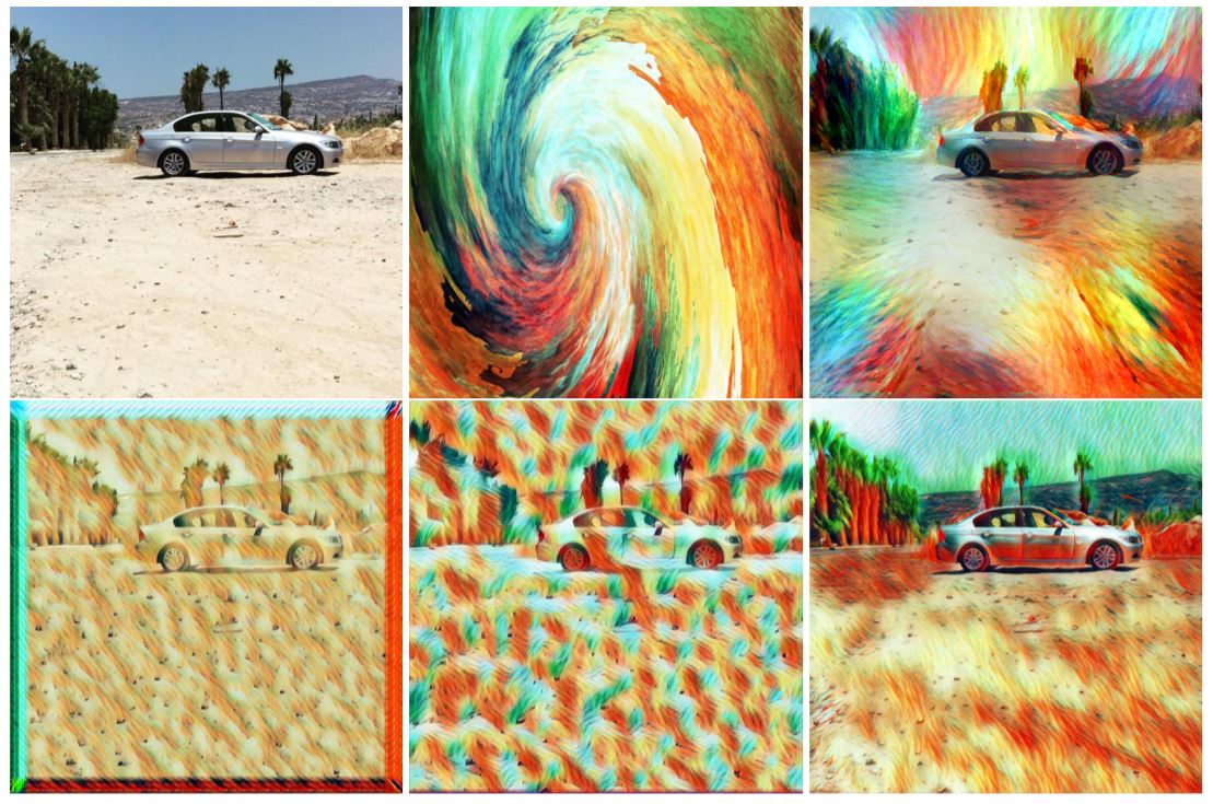
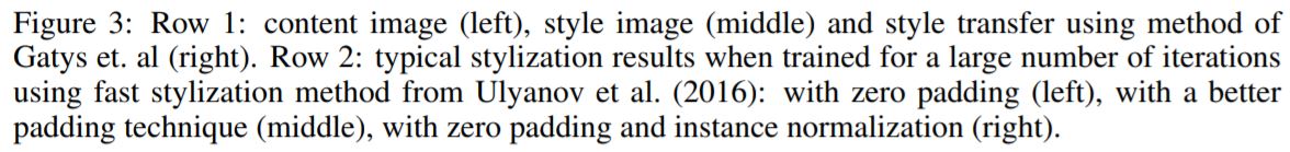
Learn a generator network \(g(x,z)\) that can apply to a given input image \(x\) the style of another \(x_0\). \(g\) is a convolutional neural network learned from examples \(x_t\) by solving

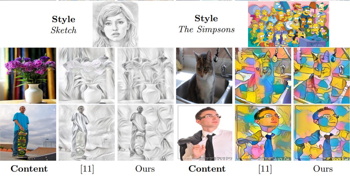
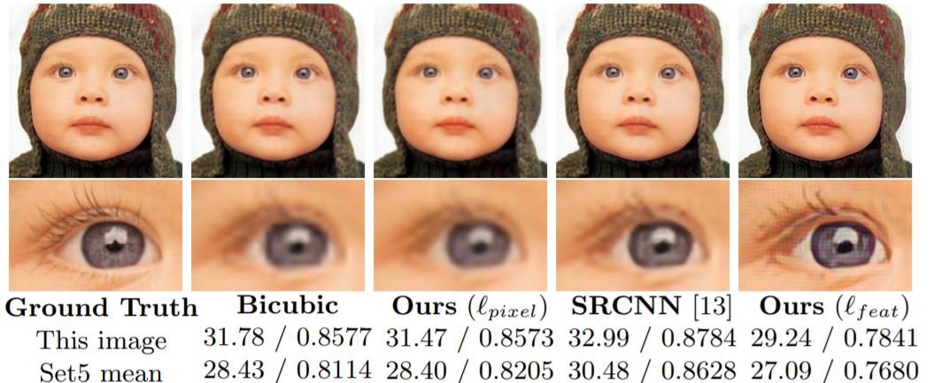
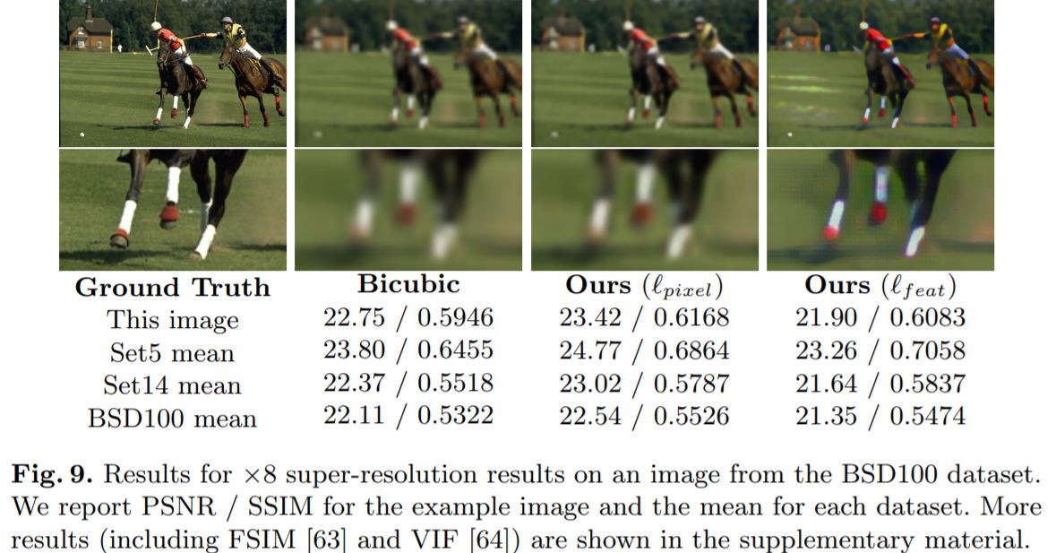
Perceptual Losses for Real-Time Style Transfer and Super Resolution

Johnson, Justin and Alahi, Alexandre and Fei-Fei, Li : 2016
Source

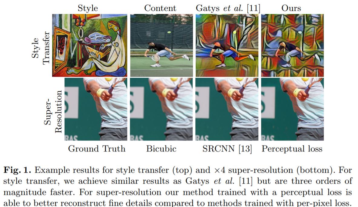
The system consists of two components : image transformation network \(f_W\)(deep resnet with encoder-decoder scheme parameterized by weights \(W\)) and a loss network \(\phi\) that is used to define several loss functions \(l_i,...l_k\).
The optimization problem becomes,

Uses the loss network \(\phi\) to define a feature reconstruction loss \(l_{feat}^{\phi}\) and style reconstruction loss \(l_{style}^{\phi}\) that measures differences in content and style between images.
Simple loss functions : In addition to the perceptual losses discussed above(and described earlier), two simple loss functions that depend only on low level pixel information are used.
Pixel Loss : Can only be used when ground truth is available.
Total Variation Regularization : to encourage spatial smoothness.
Implementation* : https://github.com/jcjohnson/fast-neural-style

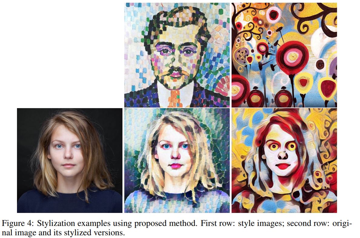
Stylizing Face Images via Multiple Exemplars

Yibing Song, Linchao Bao, Shengfeng He, Qingxiong Yang, Ming-Hsuan Yang : Aug 2017
Source

• Existing methods using a single exemplar lead to inaccurate results when the exemplar does not contain sufficient stylized facial components for a given photo.
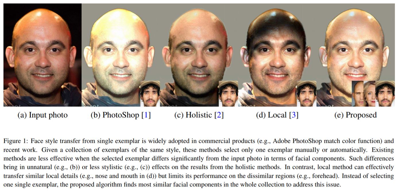
• Proposes a style transfer algorithm in which a Markov random field is used to incorporate patches from multiple exemplars. The proposed method enables the use of all stylization information from different exemplars.
  
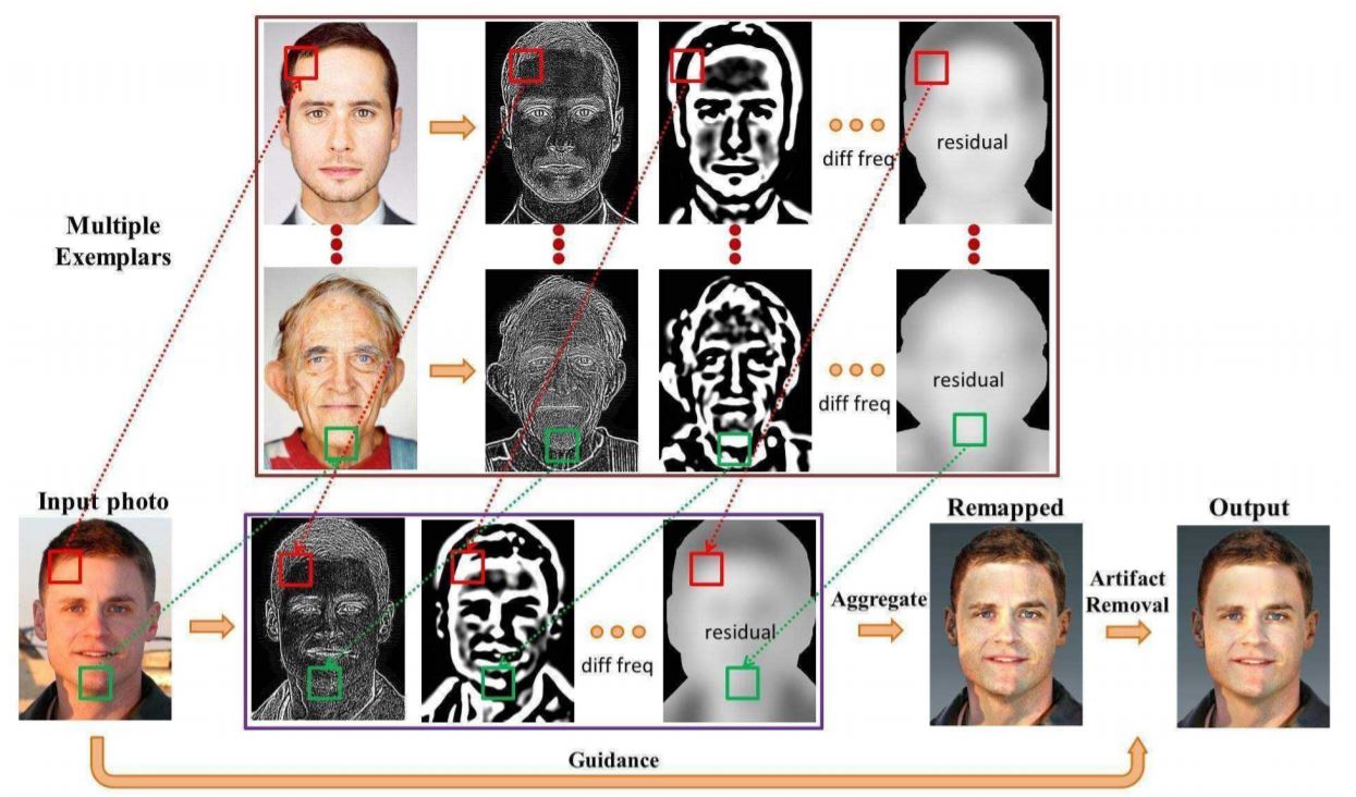
• And, proposes an artifact removal methods based on an edge-preserving filter. It removes the artifacts introduced by inconsistent boundaries of local patches stylized from different exemplars.
• In addition to visual comparison conducted by existing methods, performs quantitative evaluations using both objective and subjective metrics to demonstrate effectiveness of the proposed method.