Contents:
Chapter 2: Divide-and-Conquer Algorithms
The divide and conquer strategy solves a problem by
1. Breaking it into sub-problems that are themselves smaller instances of the same type of problem.
2. Recursively solving these problems.
3. Appropriately combining their results.
Multiplication
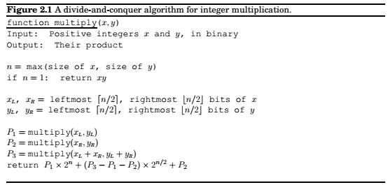
For multiplying two n-bit integers x and y.
\(x = \bbox[5px, border:2px solid black]{ x_L } \quad \bbox[5px, border:2px solid black]{ x_R } = 2^{n/2}x_L + x_R\)
\(y = \bbox[5px, border:2px solid black]{ y_L } \quad \bbox[5px, border:2px solid black]{ y_R } = 2^{n/2}y_L + y_R\)
then, \(xy = (2^{n/2}x_L + x_R)(2^{n/2}y_L + y_R) = 2^nx_Ly_L + 2^{n/2}(x_Ly_R + x_Ry_L) + x_Ry_R\)
Now, we can compute xy by evaluating the RHS. Addition and multiplication by \(2^n\) are linear time. Rest of the 4 multiplications can be done by recursively applying this algorithm.
So, \(T(n) = 4T(n/2) + O(n)\).
Which results in \(O(n^2)\).
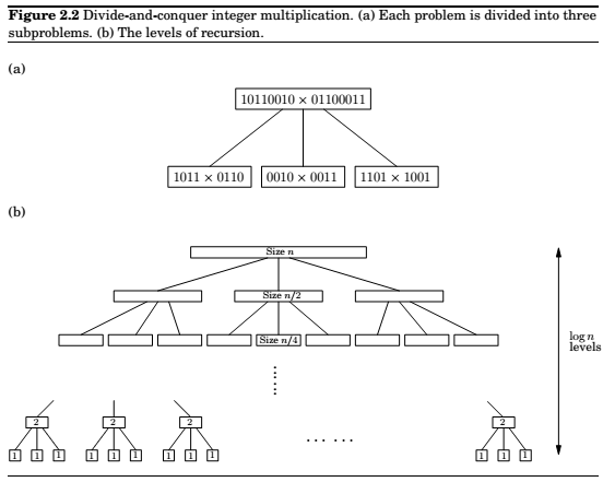
By expanding the middle term, we can do with just three calculations, \(x_Ly_L , x_Ry_R, (x_L+x_R)(y_L+y_R)\).
since,
\(x_Ly_R + x_Ry_L = (x_L + x_R ) (y_L + y_R ) - x_Ly_L – x_Ry_R\).
Resulting algorithm would then be
\(T(n) = 3T(n/2) + O(n)\), which is \(O(n^{1.59})\)
Height of the tree \(= \log_2 n\), since the length of the sub-problem gets halved at every level.
Branching factor = 3.
So, at any level k we will have \(3^k\) to solve each of size \(n/2^k\).
Therefore, time spent at level k is, \(3^k \times O(\frac n {2^k}) = (\frac 3 2)^k \times O(n)\)
Which is a geometric series. So, the sum then approximates to the last term of the series.
That is \(O(3^{\log_2 n})\), which can be written as \(O(n^{\log_2 3})\), which is about \(O(n^{1.59})\).
Can we do better ??? using Fast Fourier Transforms discussed later.
Recurrence relations
Consider this recurrence tree.
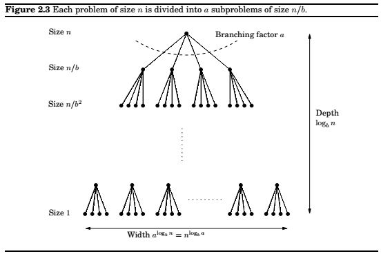
Master's Theorem :
If \(T(n) = aT(\lceil n/b \rceil) + O(n^d)\) for some constants \(a > 0, b > 1\), and \(d \ge 0\), then
Mergesort
Sort an array by recursively sorting each half and merging the results.

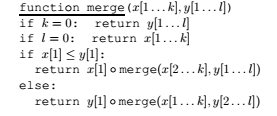
Since merge does constant amount of work per recursive call, overall time is
Here is an iterative version using a Queue.

Medians
Median = 50th percentile of a list of numbers.
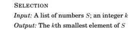
A randomized divide-and-conquer algorithm for selection
For any number v, Split S into three categories: elements smaller than v \((S_L)\), equal to v \((S_v)\) , greater than v \((S_R)\) , then
The three sub-lists can be computed in linear time, even in place.
How to pick v ? Randomly from S.

Matrix multiplication

Symbolically,
This implies the algorithm to be \(O(n^3)\)
Enter divide-and-conquer.
Divide the matrices X and Y into 4 blocks.
,
Then, their product can be expressed as,
Total running time can be described as,
\(T(n) = 8T(n/2) + O(n^2), \text{ which is again } O(n^3)\).
Turns out you can do this,
where,
\(P_1 = A(F-H) \quad\quad P_5 = (A+D)(E+H)\)
\(P_2 = (A+B)H \quad\quad P_6 = (B-D)(G+H)\)
\(P_3 = (C+D)E \quad\quad P_7 = (A-C)(E+F)\)
\(P_4 = D(G-E)\)
The new running time is, \(T(n) = 7T(n/2) + O(n^2), \text{which is } O(n^{\log_2 7}) \approx O(n^{2.81})\)
Fast Fourier transform
Next target, Polynomials.
The general solution for polynomial multiplication works in \(\theta(d^2)\) time, where \(d\) is the degree of polynomials.
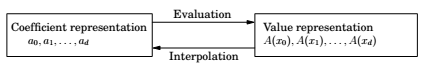
An alternative representation of polynomials.
Fact : A degree-d polynomial is uniquely characterized by its values at any \(d+1\) distinct points.
So, we can specify a degree-d polynomial
by any one of the following,
1. Its coefficients, \(a_0, a_1,..., a_d\)
2. The values \(A(x_0), A(x_1), ..., A(x_d)\)
Now, taking in consideration the second form, the product has a degree \(2d\), and is completely determined by its values at \(2d+1\) points.
Since, those values are just products of the two polynomials at the given point. Thus, polynomial multiplication takes linear time in the value representation.

Evaluation by divide-and-conquer
The Trick : Choose the n points to be selected as positive-negative pairs, then the computations needed to be done overlap a lot.
Specifically,
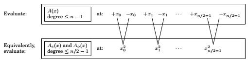
if we could then recurse, we would have,
But, recursing it at the second level and beyond seems impossible. Unless, of-course we use complex numbers.
To get positive-negative pairs at subsequent levels, we can use the roots of \(z^n = 1\)
Which are, \(1, \omega, \omega^2, ... \omega^{n-1}, \text{ where, } \omega = e^{2\pi i/n}\)
So, if we choose these numbers, at every successive level of recursion we have pairs of positive-negative numbers

Interpolation
, and
Details left,, See Fourier basis
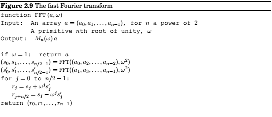
A closer look at the fast Fourier Transform
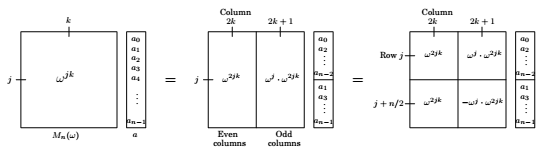
The FFT takes as input a vector \(a = (a_0, ... a_{n-1})\) and a complex number \(\omega\) whose powers are the complex root of unity.
It multiplies this vector with the Matrix \(M_n(\omega)\), which has \((j, k)_{th}\) entry (starting row and column count at zero) \(\omega^{jk}\).
Comments
comments powered by Disqus