Algorithms, Part 6

Contents:

Chapter 8: NP-Complete problems

Search problems

A set of problems that can not be solved in time better than an exhaustive search.

Satisfiability

SAT, is a problem of great practical importance, applications ranging from chip testing to computer design to image analysis and software engineering.
It is also a canonical hard problem.
Consider this Boolean formula in conjugative normal form,

It is a collection of clauses, each consisting of several literals, A satisfying truth assignment is an assignment of false or true to each variable, so that every clause is true.

SAT: Given a Boolean formula in CNF, either find a satisfying truth value, or report that none exist.
In the above example, no solution exists.But how we decide this in general. The number of possibilities is exponential.

A search problem is specified by an algorithm \(\mathcal C\) that takes two inputs, \(I\) and a proposed solution \(S\), and runs in time polynomial in \(|I|\). We say \(S\) is a solution to \(I\) if and only if \(\mathcal C(I,S) = true\).

Horn formula. If all clauses contain at most one positive literal, then the Boolean formula is called a Horn formula, and a satisfying truth assignment can be found by the greedy algorithm in Section 5.3.
Alternatively, if all clauses have only two literals, then graph theory comes into play, and SAT can be solved in linear time by finding the strongly connected components of a particular graph constructed from the instance.

The traveling salesman problem

In TSP we are given \(n\) vertices \(1,...n\) and all \(n(n-1)/2\) distance between them, as well as budget \(b\).
We are asked to find a tour, a cycle that passes through every vertex exactly once, of total cost b or less, or to report that no such tour exists.
That is we seek a permutation of the vertices such that when they are toured in this order, the total distance covered is at most b:

We have defined TSP as a search problem, when in reality it is an optimization problem, in which the shortest path is sought.
The reason is, the framework for search problems encompasses optimization problems like TSP in addition to true search problems like SAT.
This does not change its difficulty at all, because the two versions reduce to one another.

Euler and Rudrata

When can a graph be drawn without lifting the pencil from the paper?
If and only if

• the graph is connected and
• every vertex, with the possible exception of two vertices(the start and final vertices of the walk), has even degree.

EULER PATH: Given a graph, find a path that contains each edge exactly once, It follows from Euler's observation, and a little more thinking, that this search problem can be solved in polynomial time.
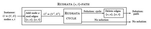
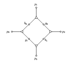
RUDRATA CYCLE: Given a graph, find a cycle that visits each vertex exactly once - or report that no such cycle exists.

Euler's problem can be solved in polynomial time, however for Rudrata's problem no polynomial solution is known.

Cuts and bisections

A cut is a set of edges whose removal leaves a graph disconnected.
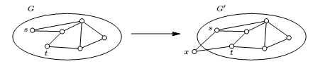
MINIMUM CUT: Given a graph and a budget \(b\), find a cut with at most \(b\) edges.
This generally leaves just a singleton vertex on one side.

BALANCED CUT: Given a graph with \(n\) vertices and a budget \(b\), partition the vertices into two sets \(S\) and \(T\) such that \(|S|, |T|>n/3\) and such that there are at most b edges between \(S\) and \(T\).
Another hard problem.

Very important application: clustering.

Integer Linear Programming

ILP: Given \(A\) and \(b\), find a nonnegative integer vector \(\mathbf x\) satisfying the inequalities \(Ax <= b\), or report that none exists.

Special case,
ZERO-ONE EQUATIONS
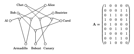
Find a vector \(\mathbb x\) of \(0\)'s and \(1\)'s satisfying \(\mathbb{Ax = 1}\), where \(\mathbb A\) is an \(m \times n\) matrix with 0-1 entries and \(\mathbb 1\) is the m-vector of all 1's.

Three-dimensional matching

BIPARTITE MATCHING: Given a bipartite graph with \(n\) nodes on each side, find a set of \(n\) disjoint edges, or decide that no such exists.

3D MATCHING: In this new setting there are 3 different sets and the compatibilities among them are specified by a triplet.
We want to find n disjoint triplets.

Independent set, vertex cover and clique

INDEPENDENT SET: Given a graph and an integer \(g\), aim is to find \(g\) vertices that are independent, that is no two of which have an edge between them.

VERTEX COVER, Given a graph and a budget \(b\), the idea is to find \(b\) vertices that cover(touch) every edge.

CLIQUE, given a graph and a goal \(g\), find a set of \(g\) vertices such that all possible edges between them are present.

Longest Path

LONGEST PATH(TAXICAB RIP-OFF) : Given a graph \(G\) with non-negative edge weights and two distinguished vertexes \(s\) and \(t\), along with a goal \(g\). We are asked to find a path from \(s\) to \(t\) with total weight at least \(g\). To avoid trivial solutions we require that the path be simple, i.e. containing no repeated vertices.

Knapsack and subset sum

KNAPSACK : we are given integer weights \(w_1,.... w_n\) and integer values \(v_1,... v_n\) for \(n\) items. We are also given a capacity \(W\) and a goal \(g\) . We seek a set of items whose total weight is at most \(W\) and whose total value is at least \(g\). If no such set exists, we should say no.

SUBSET SUM, Find a subset of a given set of integers that add up yo exactly \(W\).

NP-complete problems

Hard problems, easy problems

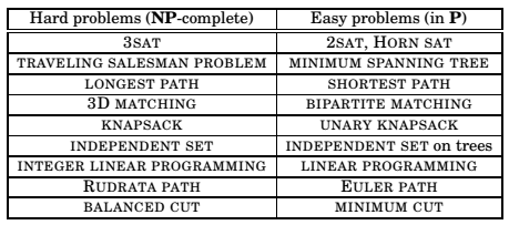
The various problems on the right can be solved by different types of algorithms, these problems are easy for a variety of reasons.
In contrast, the problems on the left are all difficult for the same reasons!
They are all the same problem, just in different disguises! They are all equivalent.

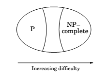
P and NP

We have already defined the search problem formally.
We denote the class of all search problems by NP.
The class of all search problems that can be solved in polynomial time is denoted by P. P = polynomial NP = nondeterministic polynomial time

Reductions, again

A reduction from search problem A to search problem B is a polynomial time algorithm f that transforms any instance I of A into an instance f(I) of B., together with another polynomial time algorithm h that maps any solution S of f(I) back into a solution h(S) of I .

A search problem is NP-complete if all other search problems reduce to it.

Factoring

The task of finding all prime factors of a given integer.
The difficulty in factoring is of a different nature than that of the other hard search problems.
Nobody believes that factoring is NP-complete.
One difference, the definition does not contain the clause, "or report that none exist". A number can always be factored into primes.
Another difference, factoring succumbs to the power of quantum computation. while other NP-complete problems do not seem to.

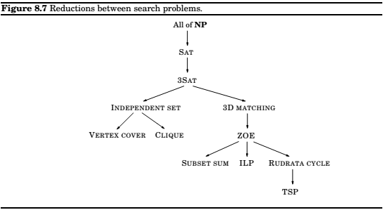
The Reductions

3SAT , example

INDEPENDENT SET,
a graph and a number g.

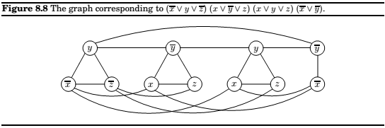
The above graph has been constructed as follows

• Graph \(G\) has a triangle for each clause(or just an edge, if the clause has two literals), with vertices labeled by the clause's literals, and has additional edges between any two vertices that represent opposite literals.
• The goal \(g\) is set to the number of clauses.

Replace,

with,

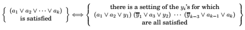
Some reductions rely on ingenuity to relate two very different problems. Others simply record the fact that one problem is a thin disguise of another. To reduce \(\mathrm{INDEPENDENT\,SET}\) to \(\mathrm{VERTEX\,COVER}\) we just need to notice that a set of nodes \(S\) is a vertex cover of graph \(G = (V,E)\) (that is \(S\) touches every edge in \(E\)) if and only if the remaining nodes, \(V-S\), are an independent set of \(G\).

Therefore, to solve an instance \((G,g)\) of \(\mathrm{INDEPENDENT\,SET}\), simple look for a vertex cover of \(G\) with \(|V|-g\) nodes. If such a vertex cover exists, then take all nodes not in it. If no such vertex cover exists, then \(G\) cannot possibly have an independent set of size \(g\).

Define the complement of a graph \(G\) to contain precisely those edges that are not in \(G\).
Then, a set of nodes is an Independent set in \(G\), if and only if it is a clique in complement of \(G\).
Therefore, the solution to both is identical.

= a boolean variable.

When we look at a \(\mathrm{ZOE}\)(like the one shown above), we are looking for a set of columns of \(A\) that, added together, make up the all-1'a vector. But if we think of the columns as binary integers(read from top to bottom), we are looking for a subset of the integers that add up to the binary integers with all 1's , i.e. 511. And this is an instance of \(\mathrm{SUBSET\,SUM}\). The reduction is complete!

Except for one detail, carry. Because of carry, n-bit binary integers can add up to \(2^n -1\),even when the sum of the corresponding vectors is not all 1's. But this is easy to fix!
Think of the column vectors not as integers in base 2, but as integers in base \(n+1\), one more than the number of columns. This way, since at most n integers are added, and all their digits are 0 and 1, there can be no carry, and our reduction works.

Chapter 9: Coping with NP completeness

Intelligent Exhaustive Search

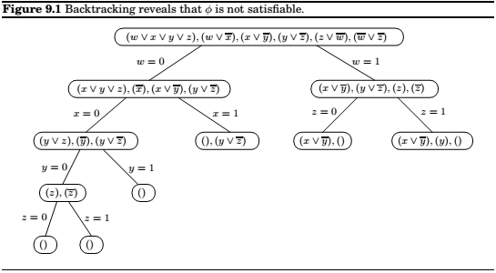
Backtracking
Based on the observation that it is often possible to reject a solution by looking at just a small part of it.

An example SAT problem.

The associated algorithm,

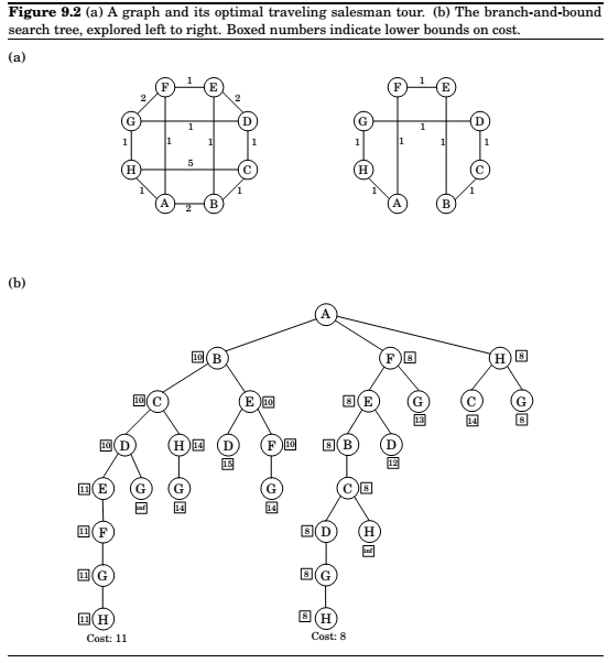
Branch and Bound

The same principle from search problems to optimization.

Let's see how this works for the travelling salesman problem in a graph \(G = (V,E)\) with edge lengths \(d_e > 0\). A partial solution is a simple path \(a \to b\) passing through some vertices \(S \subseteq V\), where \(S\) includes the endpoints \(s\) and \(b\). We can denote such a partial solution by the tuple \([a,S,b]\), infact, \(a\) will be fixed throughout the algorithm. The corresponding subproblem is to find the best completion of the tour, that is the cheapest complementary path \(b \to a\) with intermediate nodes \(V - S\). Notice that the initial problem is of the form \([a, \{a\}, a]\) for any \(a \in V\) of our choosing.
At each step of the branch-and-bound algorithm, we extend a particular partial solution \([a,S,b]\) by a single edge \((b,x)\), where \(x \in V-S\). There can be up to \(|V-S|\) ways to do this, and each of these branches leads to a subproblem of the form \([a,S\cup\{x\}, x]\).

How can we lower-bound the cost of completing a partial tour \([a,S,b]\)? Many sophisticated methods have been developed for this, but let's look at a rather simple one. The remainder of the tour consists of a path through \(V-S\), plus edges from \(a\) and \(b\) to \(V-S\). therefore, its cost is at least the sum of the following:

1. The lightest edge from \(a\) to \(V-S\).
2. The lightest edge from \(b\) to \(V-S\).
3. The minimum spanning tree of \(V-S\).

(Do you see why?) And this lower bound can be computed quickly by a minimum spanning tree algorithm.

Approximation algorithms

Approximation factor,

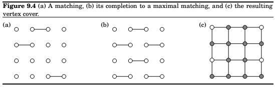
Vertex Cover

Clustering

We have some data that we want to divide into groups.

We need to define distances between these data points. These distances can be euclidean distances, or even distances as a result of similarity tests.
Assume that we have such distances and they satisfy these metric properties.

1. \(d(x,y) \geq 0\) for all \(x, y\).
2. \(d(x, y) = 0\), if and only if \(x=y\).
3. \(d(x,y) = d(y,x)\).
4. (Trianfle inequality) \(d(x,y) \leq d(x,z) + d(z,y)\)

\(\underline(k-\mathrm{CLUSTER})\)
Input: Points \(X = \{x_1...x_n\}\) with underlying distance metric \(d(\cdot,\cdot)\); integer \(k\).
Output: A partition of the points into \(k\) clusters \(C_1,...C_k\).
Goal: Minimize the diameter of the clusters,

.

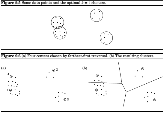
Pick any point \(\mu_1 \in X\) as the first cluster center.
for \(i = 2\) to \(k\):
\(\quad\) Let \(\mu_i\) be the point in \(X\) \(that\) \(is\) farthest from \(\mu_1...\mu_{i-1}\)
\(\quad\) (i.e., that maximizes \(min_{j<i}d(\cdot,\mu_j)\)
Create \(k\) clusters: \(C_i = {\) all \(x\inX\) whose closest center is \(\mu_i}\).

TSP
If the dustances in a TSP satisfy the triangle inequality metric, we can approximate the solution with a factor of 2 by solving the minimum spanning tree problem instead.

Knapsack

Discard any item with weight \( > W\)
Let \(v_{max} = max_iv_i\)
Rescale values \(\hat{v_i} = \lfloor v_i \cdot \frac{n}{cv_max}\rfloor\)
Run the dynamic programming algorithm with values \({\hat{v_i}}\)
Output the resulting choice of items.

The approximability hierarchy

• Those for which, like the TSP, no finite approximation ratio is possible.
• Those for which an approximation ratio is possible, but there are limits to how small this can be. \(\mathrm{VERTEX\,COVER},k-\mathrm{CLUSTER}\), and the TSP with triangle inequality belong here. (For these problems we have not established limits to their approximability, but these limits do exist, and their proofs constitute some of the most sophisticated results in this field.)
• Down below we have a more fortunate class of NP-complete problems for which approximability has no limits, and polynomial approximation algorithms with error ratios arbitarily close to zero exist. \(\mathrm{KNAPSACK}\) resides here.
• Finally, there is another class of problems, between the first two given here, for which the approximation ratio is about \(\log{n}\). \(\mathrm{SET\,COVER}\) is an example.

Local Search Heuristics

Let \(s\) be any initial solution
while there is some solution \(s'\) in the neighbourhood of \(s\)
\(\quad\) for which \(cost(s')<cost(s)\): replace \(s\) by \(s'\)
return \(s\)

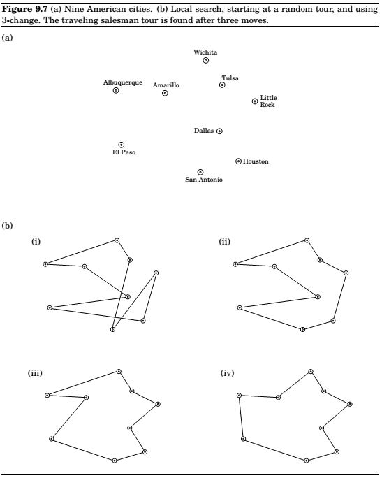
Travelling Salesman, once more

Notion of neighborhood of solutions in the search space of \((n-1)!\) different tours ?

2-change neighborhood of tour \(s\) : set of tours that can be obtained by removing two edges of \(s\) and then putting in two edges.
\(O(n^2)\) neighbors.

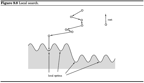
In general, the search space might be riddled with local optima, and some of them may be of very poor quality. The hope is that with a judicious choice of neighborhood structures, most local optima will be reasonable. Whether this is the reality or merely misplaced faith, it is an empirical fact that local searcg algorithms are the tp performers on a broad range of optimization problems. Let's look at another such example.

Graph partitioning

Input: An undirected graph \(G = (V,E)\) with non-negative edge weights; a real number \(\alpha \in (0,1/2)\).
Output : A partition of the vertices into two groups \(A\) and \(B\), each of size at least \(\alpha|V|\).
Goal : Minimize the capacity of the cut \((A,B)\).

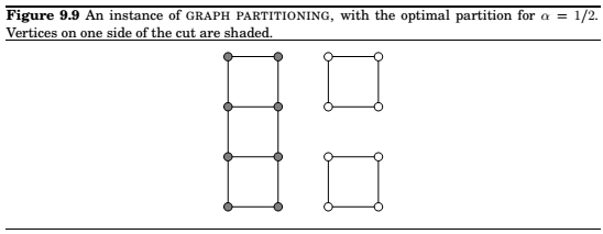
We need to decide upon a neighborhood structure for our problem, and there is one obvious way to do this. Let \((A,B)\), with \(|A|=|B|\), be a candidate solution, we will define its neighbors to be all solutions obtainable by swapping on ee pair of vertices across the cut, that is, all solutions of the form \((A-\{a\}+\{b\}, B-\{b\}+\{a\})\) where \(a\in A\) and \(b \in B\). Here's an example of a local move.

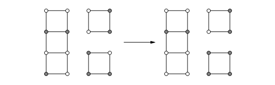
We now have a reasonable local search procedures, and we could just stop here. But there is still a lot of room for improvement in terms of the quality of the solutions produced. The search space includes some local optima that are quite far from the global solution. Here's one which has cost 2.

What can be done about such suboptimal solutions? We could expand the neighborhood size to allow two swaps at a time, but this particular bad instance would still stubbornly resist. Instead, let's look at some other generic schemes for improving local search procedures.

Dealing with local optima

Randomization and restarts

Simulated annealing,
let \(s\) be any starting solution
repeat
\(\quad\) randomly choose a solution \(s'\) in the neighborhood of \(s\)
\(\quad\) if \(\Delta=cost(s')-cost(s)\) is negative:
\(\quad\quad\) replace \(s\) by \(s'\)
\(\quad\) else:
\(\quad\) replace \(s\) by \(s'\) with probability \(e^{-\Delta/T}\).

If \(T\) is zero, this is identical to our previous local search. But if \(T\) is large, then moves that increase the cost are occasionally accepted. What value of \(T\) should be used?
The trick is to start \(T\) large and then gradually reduce it to zero. Thus initially, the local search can wander around quite freely, with only a mild preference for low-cost solutions. As time foes on, this preference becomes stronger, and the system mostly sticks to the lower-cost region of the search space, with occasional excursions out of it to escape local optima. Eventually, when the temperature drops further, the system converges on a solution.
Simulated annealing is inspired by the physics of crystallization. When a substance is to be crystallized, it starts in liquid state, with its particles in relatively unconstrained motion. Then it is slowly cooled, and as this happens, the particles gradually move into more regular configurations. This regularity becomes more and more pronounced until finally a crystal lattice is formed.
The benefits of simulated annealing comes at a significant cost: because of the changing temperature and the initial freedom of movement, many more local moves are needed until convergence. Moreover, it is quite an art to choose a good timetable by which to decrease the temperature, called annealing schedule. But in many cases where the quality of solutions improves significantly. the tradeoff is worthwhile.