Contents:
Chapter 5 : Linear Algebra
Determinants
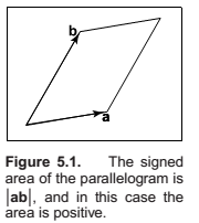
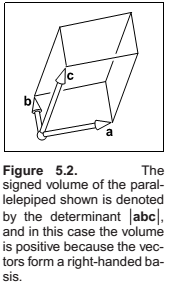
Determinants as the area of a parallelogram and volume of a parallelepiped.
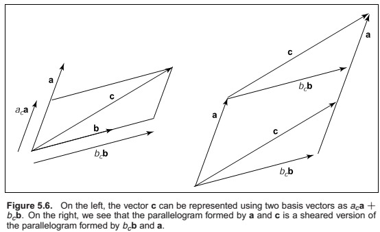
We can see from Figure 5.6 that \(|(b_c\mathbf{b}\mathbf{a})| = |c\mathbf{a}|\), because these parallelograms are just sheared versions of each other.
Solving for bc yields \(b_c =|\mathbf{ca}|/|\mathbf{ba}|\).
An analogous argument yields \(a_c =|\mathbf{bc}|/|\mathbf{ba}|\).
This is the two-dimensional version of Cramer’s rule which we will revisit soon.
Matrices
A matrix is an array of numeric elements that follow certain arithmetic rules.
Matrix Arithmetic
Product with a scalar.
Matrix addition.
Matrix multiplication. Not commutative. Associative. Distributive.
Operations on Matrices.
Identity matrix.
Inverse matrix.
Transpose of matrix,
Also,
Vector operations in Matrix form.
Special types of Matrices
- Diagonal Matrix - All non-zero elements occur along the diagonal.
- Symmetrical Matrix - Same as its transpose.
- Orthogonal Matrix - All of its rows(and columns) are vectors of length 1 and are orthogonal to each other. Determinant os such a matrix is either +1 or -1.
The idea of an orthogonal matrix corresponds to the idea of an orthonormal basis, not just a set of orthogonal vectors.
Computing with Matrices and Determinants
Determinants as areas.
Laplace's Expansion.
Computing determinants by calculating cofactors.
Computing inverses
Linear Systems
Cramer's rule,
The rule here is to take a ratio of determinants, where the denominator is \(|{\mathbf{A}}|\) and the numerator is the determinant of a matrix created by replacing a column of \(\mathbf{A}\) with the column vector \(\mathbf{b}\). The column replaced corresponds to the position of the unknown in vector \(\mathbf{x}\). For example, \(y\) is the second unknown and the second column is replaced. Note that if \(|{\mathbf{A}}| = 0\), the division is undefined and there is no solution. This is just another version of the rule that if \(\mathbf{A}\) is singular (zero determinant) then there is no unique solution to the equations.
Eigenvalues and Matrix Diagonalization
Square matrices have eigenvalues and eigenvectors associated with them. The eigenvectors are those non-zero vectors whose directions do not change when multiplied by the matrix. For example, suppose for a matrix \(\mathbf{A}\) and vector \(\mathbf{a}\), we have
This means we have stretched or compressed \(\mathbf{a}\), but its direction has not changed.
The scale factor \(\lambda\) is called the eigenvalue associated with eigenvector \(\mathbf{a}\).
If we assume a matrix has at least one eigenvector, then we can do a standard manipulation to find it. First, we write both sides as the product of a square matrix with the vector \(\mathbf{a}\):
where \(\mathbf{I}\) is an identity matrix. This can be rewritten
Because matrix multiplication is distributive, we can group the matrices:
This equation can only be true if the matrix \((\mathbf{A} − \lambda\mathbf{I})\) is singular, and thus its determinant is zero. The elements in this matrix are the numbers in \(\mathbf{A}\) except along the diagonal. Solving for \(\lambda\) requires solving an nth degree polynomial in \(\lambda\) . So we can only compute eigenvalues for matrices upto the order of 4 X 4 by analytical methods. For higher order matrices we need to use numerical solutions.
An important special case where eigenvalues and eigenvectors are particularly simple is symmetric matrices (where \(\mathbf{A} = \mathbf{A}_T\)). The eigenvalues of real symmetric matrices are always real numbers, and if they are also distinct, their eigenvectors are mutually orthogonal. Such matrices can be put into diagonal form:
where \(\mathbf{Q}\) is an orthogonal matrix and \(\mathbf{D}\) is a diagonal matrix. The columns of \(\mathbf{Q}\) are the eigenvectors of \(\mathbf{A}\) and the diagonal elements of \(\mathbf{D}\) are the eigenvalues of \(\mathbf{A}\). Putting \(\mathbf{A}\) in this form is also called the eigenvalue decomposition, because it decomposes \(\mathbf{A}\) into a product of simpler matrices that reveal its eigenvectors and eigenvalues.
Singular Value Decomposition
Here \(\mathbf{U}\) and \(\mathbf{V}\) are two, potentially different, orthogonal matrices, whose columns are known as the left and right singular vectors of \(\mathbf{A}\), and \(\mathbf{S}\) is a diagonal matrix whose entries are known as the singular values of \(\mathbf{A}\). When \(\mathbf{A}\) is symmetric and has all non-negative eigenvalues, the SVD and the eigenvalue decomposition are the same.
Also,
Chapter 6: Transformation Matrices
2D Linear Transformations
This kind of operation, which takes in a 2-vector and produces another 2-vector by a simple matrix multiplication, is a linear transformation.
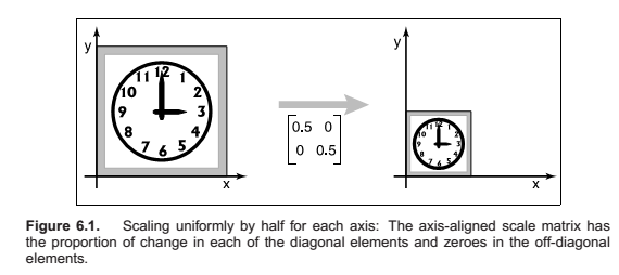
Scaling
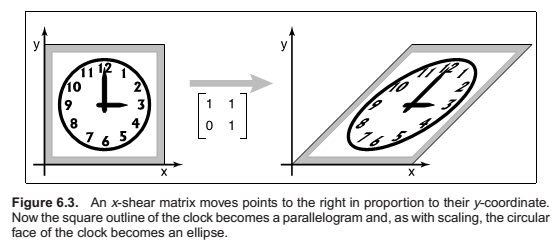
Shearing
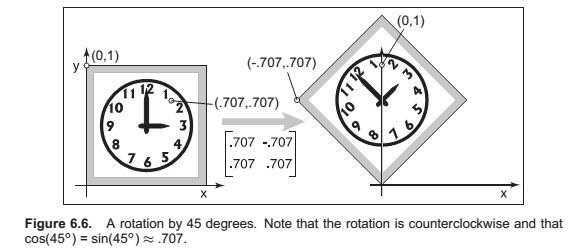
Rotation
Reflection
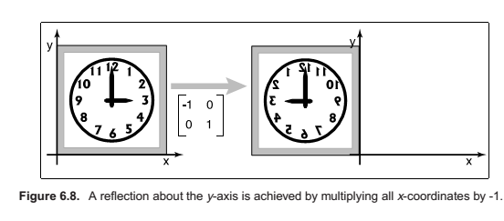
Reflection is in fact just a rotation by \(\pi\) radians.
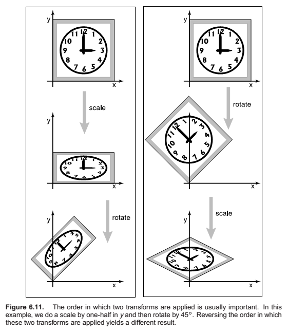
Composition and Decomposition of transforms
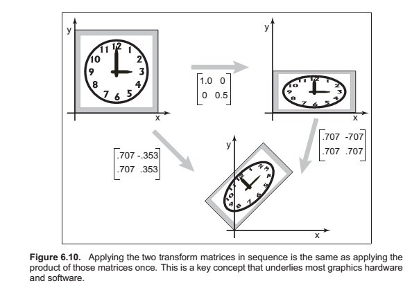
Not commutative.
Decomposition of transforms
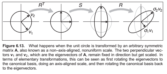
Symmetric Eigenvalue Decomposition
where \(\mathbf{R}\) is an orthogonal matrix and \(\mathbf{S}\) is a diagonal matrix; we will call the columns of \(\mathbf{R}\) (the eigenvectors) by the names \(\mathbf{v}_1\) and \(\mathbf{v}_2\), and we’ll call the diagonal entries of \(\mathbf{S}\) (the eigenvalues) by the names \(\lambda_1\) and \(\lambda_2\).
This symmetric 2 X 2 matrix has 3 degrees of freedom. One rotation angle and two scale values.
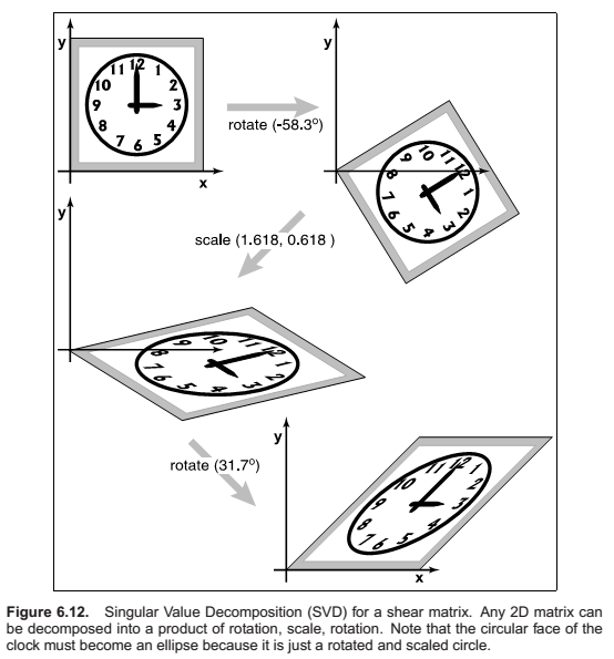
Singular value Decomposition
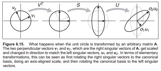
In summary, every matrix can be decomposed via SVD into a rotation times a scale times another rotation. Only symmetric matrices can be decomposed via eigenvalue diagonalization into a rotation times a scale times the inverse-rotation, and such matrices are a simple scale in an arbitrary direction. The SVD of a symmetric matrix will yield the same triple product as eigenvalue decomposition via a slightly more complex algebraic manipulation.
Paeth Decomposition of Rotations
3D Linear Transformations
Scaling
Rotation
Shear
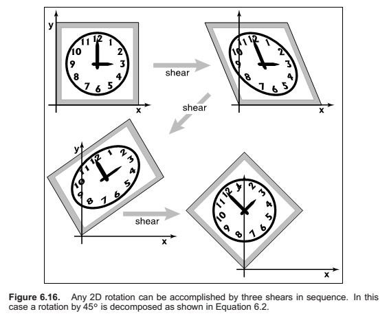
As with 2D transforms, any 3D transformation matrix can be decomposed using SVD into a rotation, scale, and another rotation. Any symmetric 3D matrix has an eigenvalue decomposition into rotation, scale, and inverse-rotation. Finally, a 3D rotation can be decomposed into a product of 3D shear matrices.
Arbitrary 3D Rotations
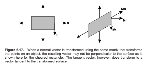
Transforming Normal Vectors
Surface normal vectors are perpendicular to the tangent plane of a surface. These normals do not transform the way we would like when the underlying surface is transformed.
Translation and Affine Transformations
For vectors that represent directions,
It is interesting to note that if we multiply an arbitrary matrix composed of scales, shears, and rotations with a simple translation (translation comes second), we get
Thus, we can look at any matrix and think of it as a scaling/rotation part and a translation part because the components are nicely separated from each other. An important class of transforms are rigid-body transforms. These are composed only of translations and rotations, so they have no stretching or shrinking of the objects. Such transforms will have a pure rotation for the \(a_{ij}\) above.
Inverses of Transformation Matrices
Coordinate Transformations
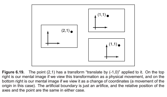
All of the previous discussion has been in terms of using transformation matrices to move points around. We can also think of them as simply changing the coordinate system in which the point is represented. For example, in Figure 6.19, we see two ways to visualize a movement. In different contexts, either interpretation may be more suitable.
For example, a driving game may have a model of a city and a model of a car. If the player is presented with a view out the windshield, objects inside the car are always drawn in the same place on the screen, while the streets and buildings appear to move backward as the player drives. On each frame, we apply a transformation to these objects that moves them farther back than on the previous frame. One way to think of this operation is simply that it moves the buildings backward; another way to think of it is that the buildings are staying put but the coordinate system in which we want to draw them—which is attached to the car—is moving. In the second interpretation, the transformation is changing the coordinates of the city geometry, expressing them as coordinates in the car’s coordinate system. Both ways will lead to exactly the same matrix that is applied to the geometry outside the car.
Coordinate frame,
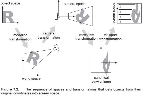
Chapter 7 : Viewing
Viewing Transformations
- A camera transformation or eye transformation, which is a rigid body transformation that places the camera at the origin in a convenient orientation. It depends only on the position and orientation, or pose, of the camera.
- A projection transformation, which projects points from camera space so that all visible points fall in the range −1 to 1 in x and y. It depends only on the type of projection desired.
- A viewport transformation or windowing transformation, which maps this unit image rectangle to the desired rectangle in pixel coordinates. It depends only on the size and position of the output image.
The Viewport Transformation
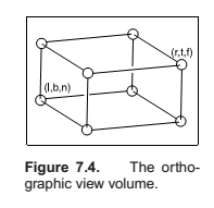
The Orthographic Projection Transformation
The Camera Transformation
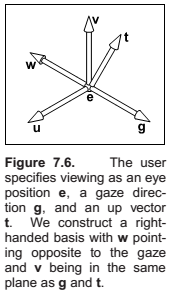
- the eye position \(\mathbf{e}\),
- the gaze direction \(\mathbf{g}\),
- the view-up vector \(\mathbf{t}\).
The algorithm:
Projective Transformations
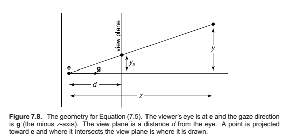
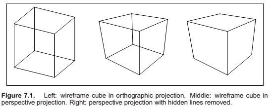
Perspective Projection
The first, second, and fourth rows simply implement the perspective equation. The third row, as in the orthographic and viewport matrices, is designed to bring the z-coordinate “along for the ride” so that we can use it later for hidden surface removal. In the perspective projection, though, the addition of a non-constant denominator prevents us from actually preserving the value of z—it’s actually impossible to keep z from changing while getting x and y to do what we need them to do. Instead we’ve opted to keep z unchanged for points on the near or far planes.
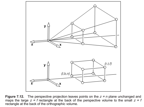

As you can see, x and y are scaled and, more importantly, divided by z. Because both n and z (inside the view volume) are negative, there are no “flips” in x and y. Although it is not obvious (see the exercise at the end of the chapter), the transform also preserves the relative order of z values between \(z = n\) and \(z = f\), allowing us to do depth ordering after this matrix is applied. This will be important later when we do hidden surface elimination.
Sometimes we will want to take the inverse of \(\mathbf{P}\), for example to bring a screen coordinate plus \(z\) back to the original space, as we might want to do for picking. The inverse is
or,
So, the full set of matrices for perspective viewing is,
The resulting algorithm is,
Some Properties of the Perspective Transform
An important property of the perspective transform is that it takes lines to lines and planes to planes. In addition, it takes line segments in the view volume to line segments in the canonical volume.
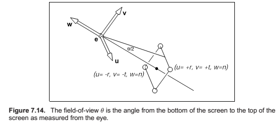
Field-of-View
Comments
comments powered by Disqus