Contents:
Chapter 8 : The Graphics Pipeline
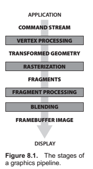
The previous several chapters have established the mathematical scaffolding we need to look at the second major approach to rendering: Drawing objects one by one onto the screen, or object-order rendering. Unlike in ray tracing, where we consider each pixel in turn and find the objects that influence its color, we'll now instead consider each geometric object in turn and find the pixels that it could have an effect on. The process of finding all the pixels in an image that are occupied by a geometric primitive is called rasterization, so object-order rendering can also be called rendering by rasterization. The sequence of operations that is required, starting with objects and ending by updating pixels in the image, is known as the graphics pipeline.
Rasterization
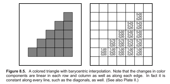
Rasterization is the central operation in object-order graphics, and the rasterizer is central to any graphics pipeline. For each primitive that comes in, the rasterizer has two jobs, it enumerates the pixels that are covered by the primitive and it interpolates values, called attributes, across the primitive - the purpose for these attributes will be clear with later examples. The output of the rasterizer is a set of fragments, one for each pixel covered by the primitive. Each fragment lives a a particular pixel and carries uts own set of attribute values.
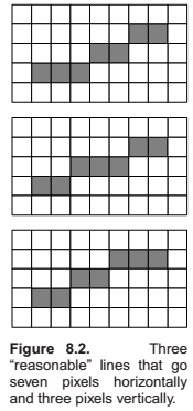
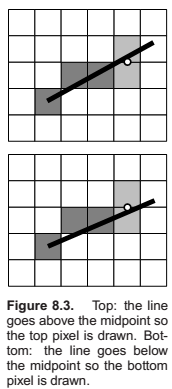
Line Drawing
Line Drawing Using Implicit Line Equations
Triangle Rasterization
Clipping
The two most common approaches for implementing clipping are
1. in world coordinates using the six planes that bound the truncated viewing pyramid,
2. in the 4D transformed space before the homogeneous divide.
This is the basic approach,.
Clipping before the transform(Option 1)
A straightforward implementation. Only question is, what are the six planes,.?
These can be inferred from the vector geometry directly or can be computed by applying inverse transform on the eight vertices of the view volume.
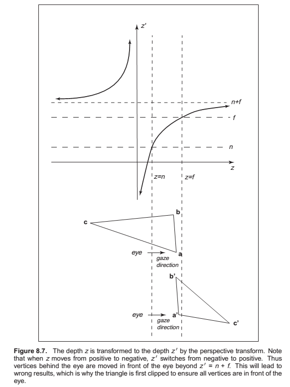
Clipping in Homogeneous Coordinates (Option 2)
Surprisingly, the option usually implemented is that of clipping in homogeneous coordinates before the divide. Here the view volume is 4D, and it is bounded by 3D volumes (hyperplanes).
Operations Before and After Rasterization
Before a primitive can be rasterized, the vertices that define it must be in screen coordinates, and the colors or other attributes that are supposed to be interpolated across the primitive must be known. Preparing this data is the job of the vertex processing stage of the pipeline. In this stage, incoming vertices are transformed by the modeling, viewing, and projection transformations, mapping them from their original coordinates into screen space (where, recall, position is measured in terms of pixels). At the same time, other information, such as colors, surface normals, or texture coordinates, is transformed as needed; we’ll discuss these additional attributes in the examples below.
After rasterization, further processing is done to compute a color and depth for each fragment. This processing can be as simple as just passing through an interpolated color and using the depth computed by the rasterizer; or it can involve complex shading operations. Finally, the blending phase combines the fragments generated by the (possibly several) primitives that overlapped each pixel to compute the final color. The most common blending approach is to choose the color of the fragment with the smallest depth (closest to the eye).
Simple 2D Drawing
The simplest possible pipeline does nothing in the vertex or fragment stages, and in the blending stage the color of each fragment simply overwrites the value of the previous one. The application supplies primitives directly in pixel coordinates, and the rasterizer does all the work. This basic arrangement is the essence of many simple, older APIs for drawing user interfaces, plots, graphs, and other 2D content. Solid color shapes can be drawn by specifying the same color for all vertices of each primitive, and our model pipeline also supports smoothly varying color using interpolation.
A Minimal 3D Pipeline
To draw objects in 3D, the only change needed to the 2D drawing pipeline is a single matrix transformation: the
vertex-processing stage multiplies the incoming vertex positions by the product of the modeling, camera,
projection, and viewport matrices, resulting in screen-space triangles that are then drawn in the same way as if
they’d been specified directly in 2D.
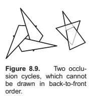
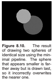
One problem with the minimal 3D pipeline is that in order to get occlusion relationships correct—to get nearer
objects in front of farther away objects— primitives must be drawn in back-to-front order. This is known as the
painter’s algorithm for hidden surface removal, by analogy to painting the background of a painting first,
then painting the foreground over it.
Using a Z-Buffer for Hidden surface removal
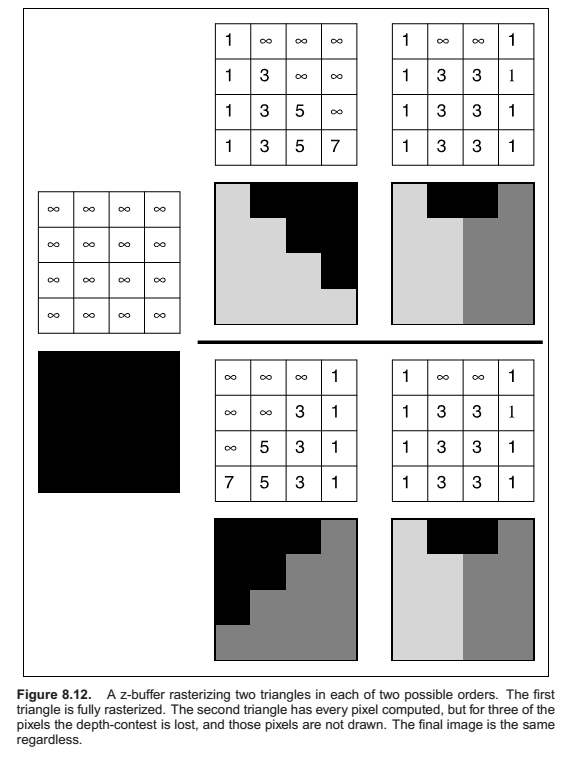
The z-buffer algorithm is implemented in the fragment blending phase, by comparing the depth of each fragment
with the current value stored in the z-buffer. If the fragment’s depth is closer, both its color and its depth
value overwrite the values currently in the color and depth buffers. If the fragment’s depth is farther away, it
is discarded. To ensure that the first fragment will pass the depth test, the z buffer is initialized to the
maximum depth (the depth of the far plane). Irrespective of the order in which surfaces are drawn, the same
fragment will win the depth test, and the image will be the same.
Per vertex Shading
One way to handle shading computations is to perform them in the vertex stage. The application provides normal vectors at the vertices, and the positions and colors of the lights are provided separately (they don’t vary across the surface, so they don’t need to be specified for each vertex). For each vertex, the direction to the viewer and the direction to each light are computed based on the positions of the camera, the lights, and the vertex. The desired shading equation is evaluated to compute a color, which is then passed to the rasterizer as the vertex color. Pervertex shading is sometimes called Gouraud shading.
Per-vertex shading has the disadvantage that it cannot produce any details in the shading that are smaller than the primitives used to draw the surface, because it only computes shading once for each vertex and never in between vertices. For instance, in a room with a floor that is drawn using two large triangles and illuminated by a light source in the middle of the room, shading will be evaluated only at the corners of the room, and the interpolated value will likely be much too dark in the center. Also, curved surfaces that are shaded with specular highlights must be drawn using primitives small enough that the highlights can be resolved.
Per-fragment Shading
To avoid the interpolation artifacts associated with per-vertex shading, we can avoid interpolating colors by performing the shading computations after the interpolation, in the fragment stage. In per-fragment shading, the same shading equations are evaluated, but they are evaluated for each fragment using interpolated vectors, rather than for each vertex using the vectors from the application.
Texture Mapping
Textures (discussed in Chapter 11) are images that are used to add extra detail to the shading of surfaces that would otherwise look too homogeneous and artificial. The idea is simple: each time shading is computed, we read one of the values used in the shading computation—the diffuse color, for instance—from a texture instead of using the attribute values that are attached to the geometry being rendered. This operation is known as a texture lookup: the shading code specifies a texture coordinate, a point in the domain of the texture, and the texture-mapping system finds the value at that point in the texture image and returns it. The texture
value is then used in the shading computation.
The most common way to define texture coordinates is simply to make the texture coordinate another vertex attribute. Each primitive then knows where it lives in the texture.
Simple Antialiasing
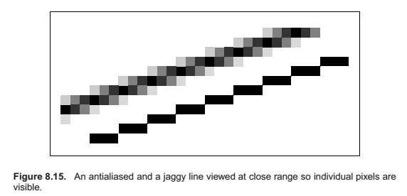
Just as with ray tracing, rasterization will produce jagged lines and triangle edges if we make an all-or-nothing determination of whether each pixel is inside the primitive or not. In fact, the set of fragments generated by the simple triangle rasterization algorithms described in this chapter, sometimes called standard or aliased rasterization, is exactly the same as the set of pixels that would be mapped to that triangle by a ray tracer that sends one ray through the center of each pixel. Also as in ray tracing, the solution is to allow pixels to be partly covered by a primitive (Crow, 1978). In practice this form of blurring helps visual quality, especially in animations. This is shown as the top line of Figure 8.15.
The easiest way to implement box-filter antialiasing is by supersampling: create images at very high resolutions and then downsample. For example, if our goal is a 256 × 256 pixel image of a line with width 1.2 pixels, we could rasterize a rectangle version of the line with width 4.8 pixels on a 1024 × 1024 screen, and then average 4 × 4 groups of pixels to get the colors for each of the 256 × 256 pixels in the “shrunken” image. This is an approximation of the actual boxfiltered image, but works well when objects are not extremely small relative to the distance between pixels.
Supersampling is quite expensive, however. Because the very sharp edges that cause aliasing are normally caused by the edges of primitives, rather than sudden variations in shading within a primitive, a widely used optimization is to sample visibility at a higher rate than shading. If information about coverage and depth is stored for several points within each pixel, very good antialiasing can be achieved even if only one color is computed. In systems like RenderMan that use per-vertex shading, this is achieved by rasterizing at high resolution: it is inexpensive to do so because shading is simply interpolated to produce colors for the many fragments, or visibility samples. In systems with per-fragment shading, such as hardware pipelines, multisample antialiasing is achieved by storing for each fragment a single color plus a coverage mask and a set of depth values.
Culling Primitives for Efficiency
The strength of object-order rendering, that it requires a single pass over all the geometry in the scene, is also a weakness for complex scenes. For instance, in a model of an entire city, only a few buildings are likely to be visible at any given time. A correct image can be obtained by drawing all the primitives in the scene, but a great deal of effort will be wasted processing geometry that is behind the visible buildings, or behind the viewer, and therefore doesn’t contribute to the final image.
Identifying and throwing away invisible geometry to save the time that would be spent processing it is known as culling.
- view volume culling : the removal of geometry that is outside the view volume;
- occlusion culling : the removal of geometry that may be within the view volume but is obscured, or occluded, by other geometry closer to the camera;
- backface culling : the removal of primitives facing away from the camera.
View Volume Culling
When an entire primitive lies outside the view volume, it can be culled, since it will produce no fragments when rasterized. If we can cull many primitives with a quick test, we may be able to speed up drawing significantly. On the other hand, testing primitives individually to decide exactly which ones need to be drawn may cost more than just letting the rasterizer eliminate them.
View volume culling, also known as view frustum culling, is especially helpful when many triangles are grouped into an object with an associated bounding volume. If the bounding volume lies outside the view volume, then so do all the triangles that make up the object. For example, if we have 1000 triangles bounded by a single sphere with center \(\mathbf{c}\) and radius \(\mathbf{r}\), we can check whether the sphere lies outside the clipping plane,
Backface Culling
When polygonal models are closed, i.e., they bound a closed space with no holes, then they are often assumed to have outward facing normal vectors as discussed in Chapter 10. For such models, the polygons that face away from the eye are certain to be overdrawn by polygons that face the eye. Thus, those polygons can be culled before the pipeline even starts.
Chapter 9 : Signal Processing
Digital Audio: Sampling in 1D
Sampling Artifacts and aliasing
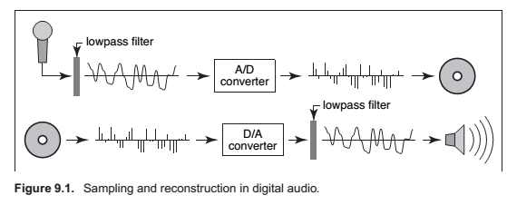
The digital audio recording chain can serve as a concrete model for the sampling and reconstruction processes that happen in graphics. The same kind of undersampling and reconstruction artifacts also happen with images or other sampled signals in graphics, and the solution is the same: filtering before sampling and filtering again during reconstruction.
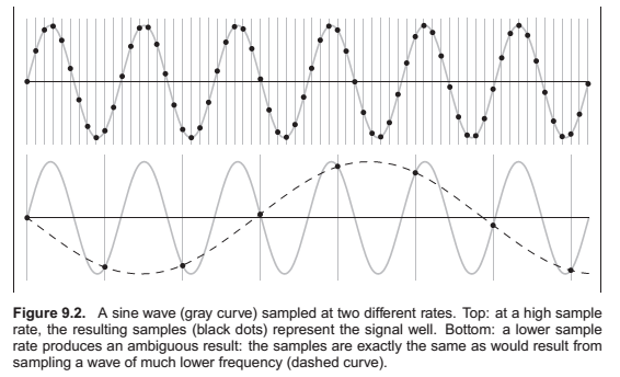
Once the sampling has been done, it is impossible to know which of the two signals—the fast or the slow sine wave—was the original, and therefore there is no single method that can properly reconstruct the signal in both cases. Because the high frequency signal is “pretending to be” a low-frequency signal, this phenomenon is known as aliasing.
Questions,..
What sample rate is high enough to ensure good results?
What kinds of filters are appropriate for sampling and reconstruction?
* What degree of smoothing is required to avoid aliasing?
Convolution
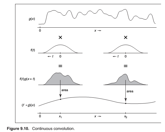
Convolution is an operation on functions: it takes two functions and combines them to produce a new function. In this book, the convolution operator is denoted by a star: the result of applying convolution to the functions \(f\) and \(g\) is \(f \star g\). We say that \(f\) is convolved with \(g\), and \(f \star g\) is the convolution of \(f\) and \(g\).
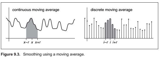
Moving Averages
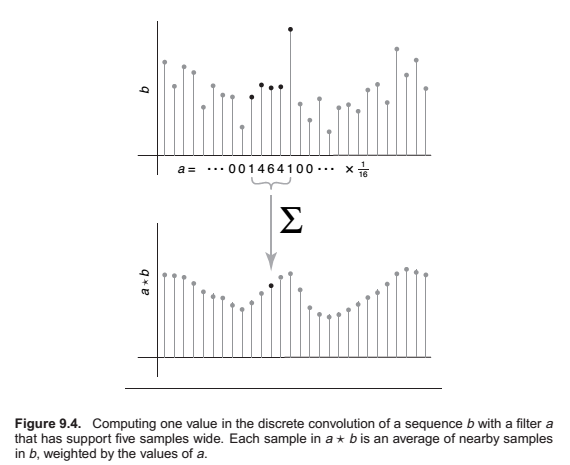
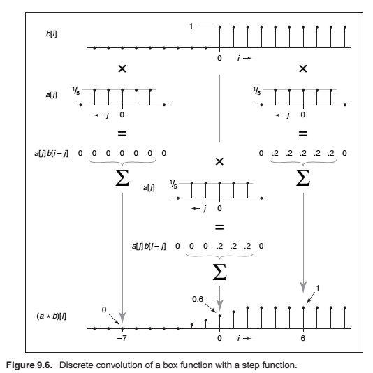
Discrete Convolution
Convulution Filters
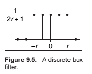
Box filter,
Properties of Convolution
- commutative: \((a b)[i] = (b a)[i]\)
- associative: \((a (b c))[i] = ((a b) c)[i]\)
- distributive: \((a (b + c))[i] = (a b + a c)[i]\)
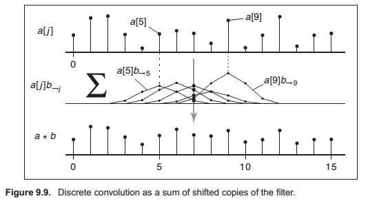
Convolution as a Sum of Shifted Filters
Convolution with Continuous Functions
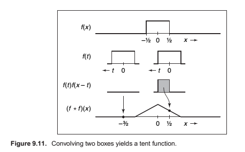
Example (Convolution of two box functions).
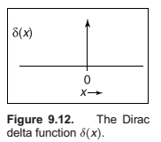
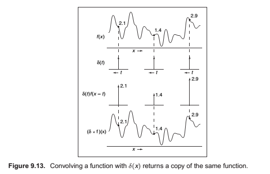
The Dirac Delta Function
In discrete convolution, we saw that the discrete impulse d acted as an identity: d a = a. In the continuous case, there is also an identity function, called the Dirac impulse or Dirac delta function, denoted
\(\delta(x)\).
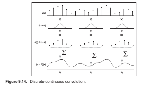
Discrete-Continuous Convolution
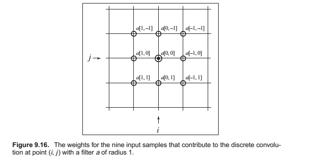
Convolution in More Than One Dimension
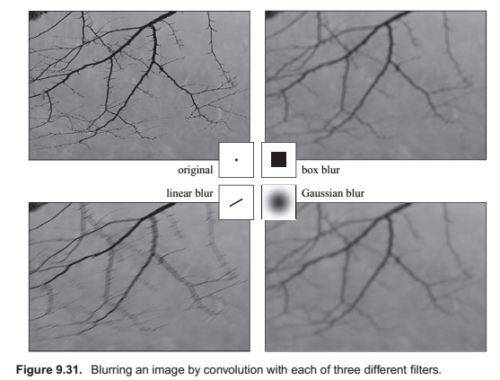
Convolution Filters
A Gallery of Convolution Filters
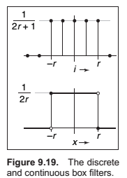
The Box Filter
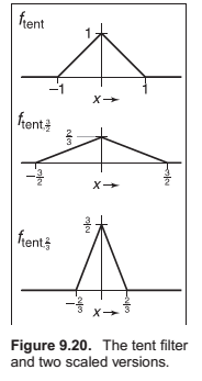
The Tent Filter.
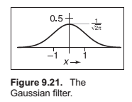
The Gaussian Filter.
Also known as the normal distribution is an important filer theoretically and practically.
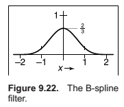
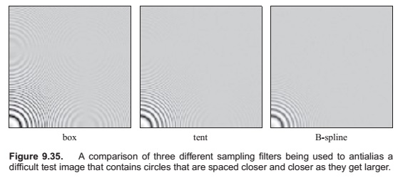
The B-spline cubic filter.
The blending function for spline curves. It has continuos first and second derivatives -- that is, it is \(C_2\)
A more concise way of defining this filter is \(F_B = f_{box} X f_{box} X f_{box} X f_{box}\).
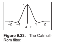
The Catmull-RomCubic Fiilter.
The Mitchell-Netravali Cubic Filter.

Properties of Filters
A continuous filter has a degree of continuity, which is the highest-order derivative that is defined everywhere
Separable Filters
Example,
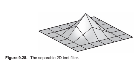
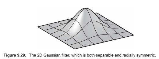
Notice that this is (up to a scale factor) the same function we would get if we revolved the 1D Gaussian around the origin to produce a circularly symmetric function. The property of being both circularly symmetric and separable at the same time is unique to the Gaussian function. The profiles along the coordinate axes are Gaussians, but so are the profiles along any direction at any offset from the center.

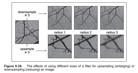
This savings has great significance for large filters. Filtering an \(m \times n\) 2D image with a filter of radius \(r\) in the general case requires computation of \((2r+1)^2\) products per pixel, while filtering the image with a separable filter of the same size requires \(2(2r + 1)\) products (at the expense of some intermediate storage). This change in asymptotic complexity from \(O(r^2)\) to \(O(r)\) enables the use of much larger filters.
The algorithm is,
Signal Processing for Images
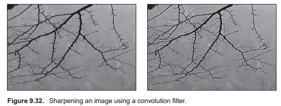
Image Filtering Using Discrete Filters
Antialiasing in Image Sampling
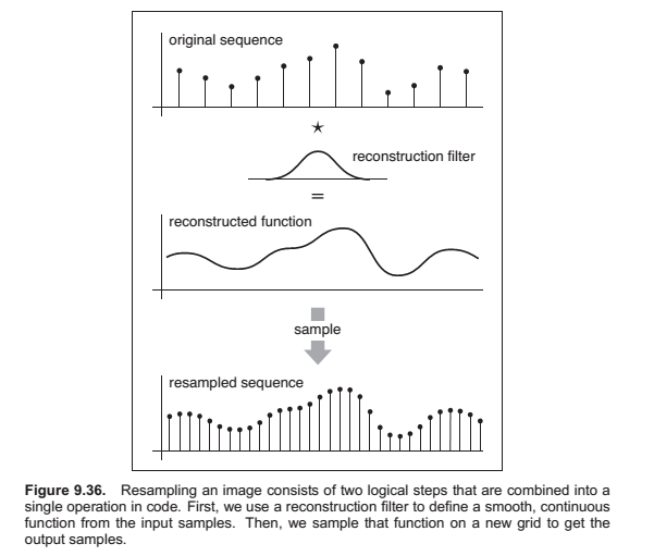
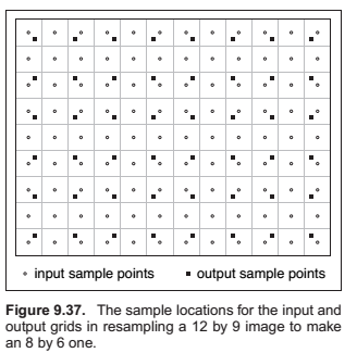
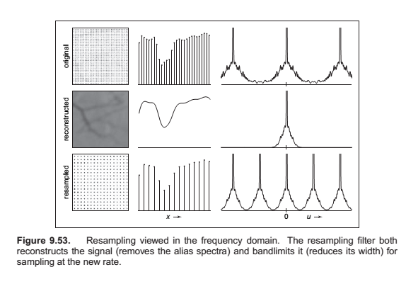
Reconstruction and Resampling

Sampling Theory
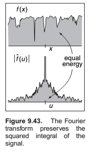
When a function \(f\) is expressed in this way, this weight, which is a function of the frequency \(u\), is called the Fourier transform of \(f\), denoted \(\hat f\).
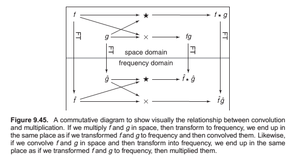
Convolution and the Fourier Transform
A Gallery of Fourier Transforms
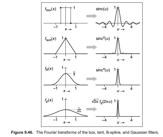
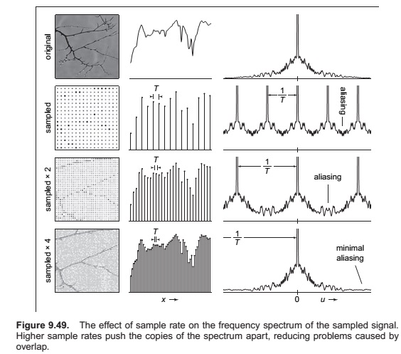
Sampling and Aliasing
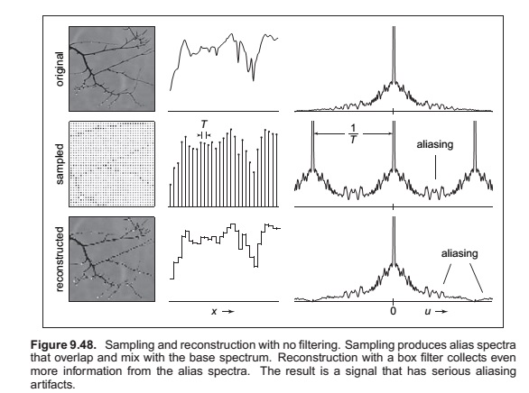
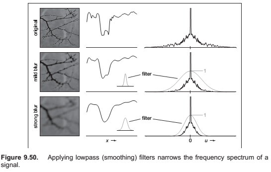
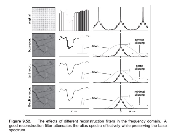
Preventing Aliasing in Sampling

Comments
comments powered by Disqus