Contents:
Chapter 12 : Data Structures for Graphics
Triangle Meshes
Most real-world models are composed of complexes of triangles with shared vertices. These are usually known as triangular meshes, triangle meshes, or triangular irregular networks (TINs) and handling them efficiently is crucial to the performance of many graphics programs.
The minimum information required for a triangle mesh is a set of triangles (triples of vertices) and the positions (in 3D space) of their vertices. But many, if not most, programs require the ability to store additional data at the vertices, edges, or faces to support texture mapping, shading, animation, and other operations. Vertex data is the most common: each vertex can have material parameters, texture coordinates, irradiances—any parameters whose values change across the surface. These parameters are then linearly interpolated across each triangle to define a continuous function over the whole surface of the mesh. However, it is also occasionally important to be able to store data per edge or per face.
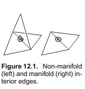
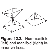
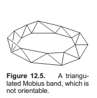
Mesh Topology
- Every edge is shared by exactly two triangles.
- Every vertex has a single, complete loop of triangles around it.
Indexed Mesh Storage
Triangle {
     vector3 vertexPosition[3]
}
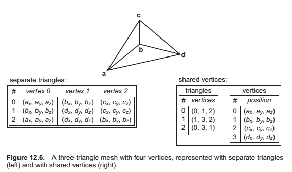
Triangle {
     Vertex v[3]
}
Vertex {
     vector3 position // or other vertex data
}
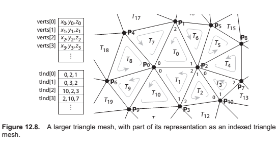
Indexed triangle mesh
IndexedMesh {
     int tInd[nt][3]
     vector3 verts[nv]
}
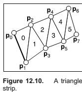
Triangle Strips and Fans
Data Structures for Mesh Connectivity
Indexed meshes, strips, and fans are all good, compact representations for static meshes. However, they do not readily allow for meshes to be modified. In order to efficiently edit meshes, more complicated data structures are needed to efficiently answer queries such as:
Given a triangle, what are the three adjacent triangles?
Given an edge, which two triangles share it?
Given a vertex, which faces share it?
Given a vertex, which edges share it?
The most straightforward, though bloated, implementation would be to have three types, Vertex, Edge, and Triangle, and to just store all the relationships directly:
Triangle {
     Vertex v[3]
     Edge e[3]
}
Edge {
     Vertex v[2]
     Triangle t[2]
}
Vertex {
     Triangle t[]
     Edge e[]
}
The fixed-size arrays in the Edge and Triangle classes suggest that it will be more efficient to store the connectivity information there. In fact, for polygon meshes, in which polygons have arbitrary numbers of edges and vertices, only edges have fixed-size connectivity information, which leads to many traditional mesh data structures being based on edges. But for triangle-only meshes, storing connectivity in the (less numerous) faces is appealing.
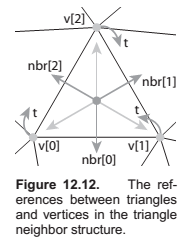
The Triangle-Neighbor Structure
Triangle {
     Triangle nbr[3];
     Vertex v[3];
}
Vertex {
     // ... per-vertex data ...
     Triangle t; // any adjacent tri
}
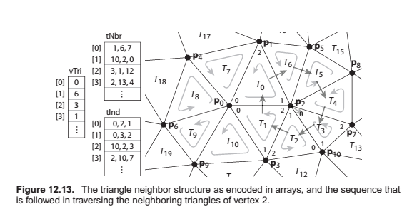
Mesh {
     // ... per-vertex data ...
     int tInd[nt][3]; // vertex indices
     int tNbr[nt][3]; // indices of neighbor triangles
     int vTri[nv]; // index of any adjacent triangle
}
TrianglesOfVertex(v) {
     t = v.t
     do {
          find i such that (t.v[i] == v)
          t = t.nbr[i]
     } while (t != v.t)
}
The Winged-Edge structure
Edge {
     Edge lprev, lnext, rprev, rnext;
     Vertex head, tail;
     Face left, right;
}
Face {
     // ... per-face data ...
     Edge e; // any adjacent edge
}
Vertex {
     // ... per-vertex data ...
     Edge e; // any incident edge
}
The Half-Edge Structure
HEdge {
     HEdge pair, next;
     Vertex v;
     Face f;
}
Face {
     // ... per-face data ...
     HEdge h; // any h-edge of this face
}
Vertex {
     // ... per-vertex data ...
     HEdge h; // any h-edge pointing toward this vertex
}
Scene Graphs
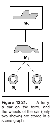
As with the pendulum, each object should be transformed by the product of the matrices in the path from the root to the object:
- ferry transform using \(M_0\)
- car body transform using \(M_0M_1\)
- left wheel transform using \(M_0M_1M_2\)
- left wheel transform using \(M_0M_1M_3\)
An efficient implementation can be achieved using a matrix stack, a data structure supported by many APIs. A matrix stack is manipulated using push and pop operations that add and delete matrices from the right-hand side of a matrix product.
For example, calling:
creates the active matrix \(\mathbf M = \mathbf M_0 \mathbf M_1 \mathbf M_2\). A subsequent call to pop() strips the last matrix added so that the active matrix becomes \(\mathbf M = \mathbf M_0 \mathbf M_1\). Combining the matrix stack with a recursive traversal of a scene graph gives us:
Spatial Data Structures
Bounding Boxes
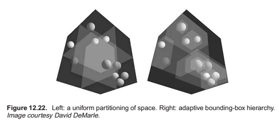
Hierarchical Bounding Boxes
There are many ways to build a tree for a bounding volume hierarchy. It is convenient to make the tree binary, roughly balanced, and to have the boxes of sibling subtrees not overlap too much. A heuristic to accomplish this is to sort the surfaces along an axis before dividing them into two sublists.
The quality of the tree can be improved by carefully choosing AXIS each time. One way to do this is to choose the axis such that the sum of the volumes of the bounding boxes of the two subtrees is minimized. This change compared to rotating through the axes will make little difference for scenes composed of isotopically distributed small objects, but it may help significantly in less well-behaved scenes. This code can also be made more efficient by doing just a partition rather than a full sort.
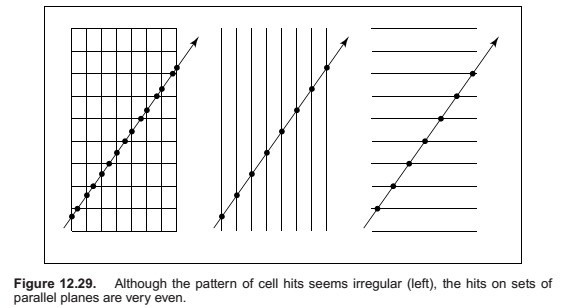
Uniform Spatial Subdivision
- In hierarchical bounding volumes, each object belongs to one of two sibling nodes, whereas a point in space may be inside both sibling nodes.
- In spatial subdivision, each point in space belongs to exactly one node, whereas objects may belong to many nodes.
The grid itself should be a subclass of surface and should be implemented as a 3D array of pointers to surface. For empty cells these pointers are NULL. For cells with one object, the pointer points to that object. For cells with more than one object, the pointer can point to a list, another grid, or another data structure, such as a bounding volume hierarchy.
Axis-Aligned Binary Space Partitioning
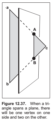
A node in this structure contains a single cutting plane and a left and right subtree. Each subtree contains all the objects on one side of the cutting plane. Objects that pass through the plane are stored in in both subtrees. If we assume the cutting plane is parallel to the \(yz\) plane at \(x = D\), then the node class is:
class bsp-node subclass of surface
     virtual bool hit(ray e + td, real t0, real t1, hit-record rec)
     virtual box bounding-box()
     surface-pointer left
     surface-pointer right
     real D
BSP Trees for Visibility
If we are making many images of a fixed scene composed of planar polygons, from different viewpoints—as is often the case for applications such as games— we can use a binary space partitioning scheme closely related to the method for ray intersection discussed in the previous section. The difference is that for visibility sorting we use non–axis-aligned splitting planes, so that the planes can be made coincident with the polygons. This leads to an elegant algorithm known as the BSP tree algorithm to order the surfaces from front to back. The key aspect of the BSP tree is that it uses a preprocess to create a data structure that is useful for any viewpoint. So, as the viewpoint changes, the same data structure is used without change.
Overview of BSP Tree Algorithm
The BSP tree algorithm is an example of a painter’s algorithm. A painter’s algorithm draws every object from back-to-front, with each new polygon potentially overdrawing previous polygons.
Building the Tree
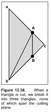
A precision problem that will plague a naive implementation occurs when a vertex is very near the splitting plane. For example, if we have two vertices on one side of the splitting plane and the other vertex is only an extremely small distance on the other side, we will create a new triangle almost the same as the old one, a triangle that is a sliver, and a triangle of almost zero size. It would be better to detect this as a special case and not split into three new triangles. One might expect this case to be rare, but because many models have tessellated planes and triangles with shared vertices, it occurs frequently, and thus must be handled carefully. Some simple manipulations that accomplish this are:
Cutting Triangles
Optimizing the Tree
Mostly depends upon the order or triangle being added.
Tiling Multidimensional Arrays
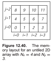
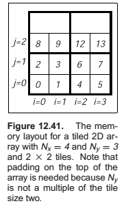
One-Level Tiling for 2D Arrays
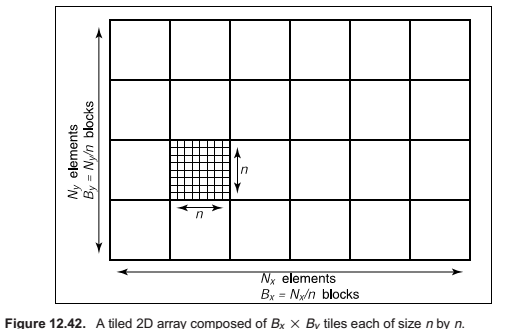
Thus the full formula for finding the 1D index element \((x, y)\) in an \(N_x \times N_y\) array with \(n \times n\)
tiles is,
This expression contains many integer multiplication, divide and modulus operations, which are costly on some processors. When \(n\) is a power of two, these operations can be converted to bitshifts and bitwise logical operations. However, as noted above, the ideal size is not always a power of two.
However, there is a simple solution; note that the index expression can be written as
where,
We tabulate \(F_x\) and \(F_y\), and use \(x\) and \(y\) to find the index into the data array. These tables will consist of \(N_x\) and \(N_y\) elements, respectively. The total size of the tables will fit in the primary data cache of the processor, even for very large data set sizes.
Chapter 13 : More Ray Tracing
If you start with a bruteforce ray intersection loop, you’ll have ample time to implement an acceleration structure while you wait for images to render.
Transparency and Refraction
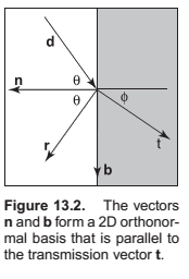
Snell's Law,
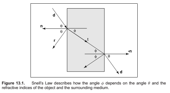
Since we can describe \(\mathbf d\) in the same basis, and \(\mathbf d\) is known, we can
solve for \(\mathbf b\):
This means we can solve for \(\mathbf t\) with known variables,
Shilck approximations for Fresnel equations,
where \(R_0\) is the reflactance at normal incidence:

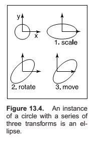
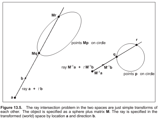
Instancing
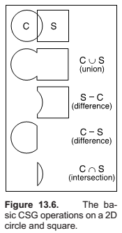
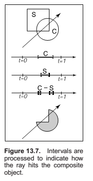
Constructive Solid Geometry
Distribution Ray Tracing
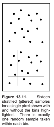
Antialiasing
For a code hat samples \(n \times n\) samples across each pixel:
This is called regular sampling.
One potential problem with taking samples in a regular pattern within a pixel is that regular artifacts such as moir´e patterns can arise.
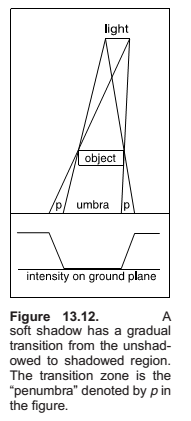
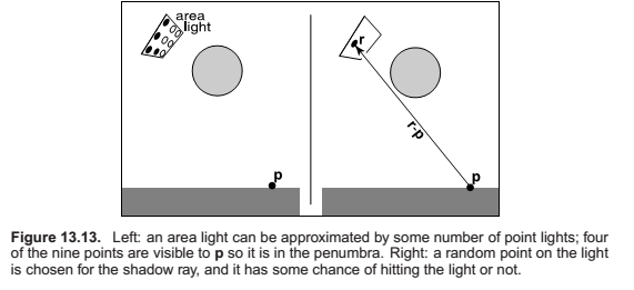
Soft Shadows
A Shuffle routine,
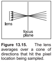
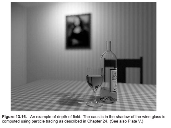
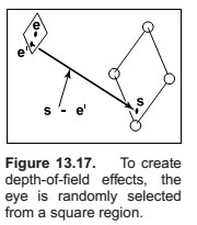
Depth of Field
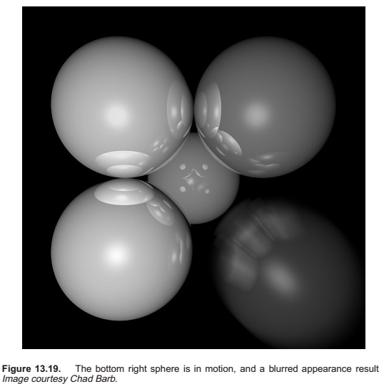
Motion Blur
Comments
comments powered by Disqus