Contents:
Chapter 10 : Surface Shading
Diffuse Shading
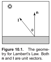
Many objects in the world have a surface appearance loosely described as “matte,” indicating that the object is not at all shiny. Examples include paper, unfinished wood, and dry unpolished stones. To a large degree, such objects do not have a color change with a change in viewpoint. For example, if you stare at a particular point on a piece of paper and move while keeping your gaze fixed on that point, the color at that point will stay relatively constant. Such matte objects can be considered as behaving as Lambertian objects.
Lambertian Shading Model
Ambient Shading
Vertex-Based Diffuse Shading
If we apply the above equation to an object made up of triangles, it will typically have a faceted appearance. Often, the triangles are an approximation to a smooth surface. To avoid the faceted appearance, we can place surface normal vectors at the vertices of the triangles (Phong, 1975), and apply Equation (10.3) at each of the vertices using the normal vectors at the vertices (see Figure 10.4). This will give a color at each triangle vertex, and this color can be interpolated using the barycentric interpolation described in Section 8.1.2.
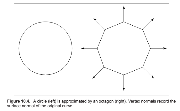
One problem with shading at triangle vertices is that we need to get the normals from somewhere. Many models will come with normals supplied. If you tessellate your own smooth model, you can create normals when you create the triangles. If you are presented with a polygonal model that does not have normals at vertices and you want to shade it smoothly, you can compute normals by a variety of heuristic methods. The simplest is to just average the normals of the triangles that share each vertex and use this average normal at the vertex. This average normal will not automatically be of unit length, so you should convert it to a unit vector before using it for shading.
Phong Shading
Some surfaces are essentially like matte surfaces, but they have highlights. Examples of such surfaces include polished tile floors, gloss paint, and whiteboards. Highlights move across a surface as the viewpoint moves. This means that we must add a unit vector e toward the eye into our equations. If you look carefully at highlights, you will see that they are really reflections of the light; sometimes these reflections are blurred. The color of these highlights is the color of the light—the surface color seems to have little effect. This is because the reflection occurs at the object’s surface, and the light that penetrates the surface and picks up the object’s color is scattered diffusely.
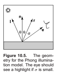
Phong Lighting Model
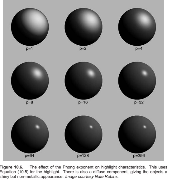
We want to add a fuzzy “spot” the same color as the light source in the right place. The center of the dot should be drawn where the direction \(e\) to the eye “lines” up with the natural direction of reflection \(r\) as shown in Figure 10.5. Here “lines up” is mathematically equivalent to “where \(\sigma\) is zero.” We would like to have the highlight have some non-zero area, so that the eye sees some highlight wherever \(\sigma\) is small.
\(p\) is the Phong Exponent.
Another heuristic can also be used here,.
Surface Normal Vector Interpolation
Smooth surfaces with highlights tend to change color quickly compared to Lambertian surfaces with the same geometry. Thus, shading at the normal vectors can generate disturbing artifacts.
These problems can be reduced by interpolating the normal vectors across the polygon and then applying Phong shading at each pixel. This allows you to get good images without making the size of the triangles extremely small.
Artistic Shading
The Lambertian and Phong shading methods are based on heuristics designed to imitate the appearance of objects in the real world.
Line Drawing
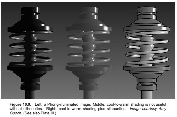
The most obvious thing we see in human drawings that we don’t see in real life is silhouettes.
draw silhouette if \(f_0(\mathbf{e})f_1(\mathbf{e}) \leq 0\).
draw crease if \((\mathbf{n}_0 · \mathbf{n}_1) \leq \text{threshold}\)
Cool-to-Warm Shading
Chapter 11 : Texture Mapping
The shading models presented in Chapter 10 assume that a diffuse surface has uniform reflectance \(c_r\). This is fine for surfaces such as blank paper or painted walls, but it is inefficient for objects such as a printed sheet of paper. Such objects have an appearance whose complexity arises from variation in reflectance properties. While we could use such small triangles that the variation is captured by varying the reflectance properties of the triangles, this would be inefficient.
Texture mapping can be classified by several different properties: 1. the dimensionality of the texture function, 2. the correspondences defined between points on the surface and points in the texture function, and 3. whether the texture function is primarily procedural or primarily a table look-up.
3D Texture Mapping
3D Stripe Textures
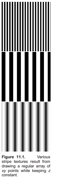
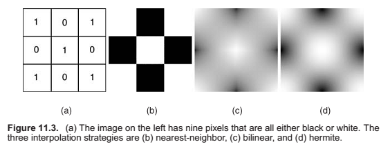
Texture Arrays
Solid Noise
Perlin noise.
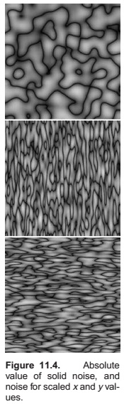
Getting a noisy appearance by calling a random number for every point would not be appropriate, because it would just be like white noise in TV static. We would like to make it smoother without losing the random quality. One
possibility is to blur white noise, but there is no practical implementation of this. Another possibility is to make a large lattice with a random number at every lattice point, and then interpolate these random points for new points
between lattice nodes; this is just a 3D texture array as described in the last section with random numbers in the array. This technique makes the lattice too obvious. Perlin used a variety of tricks to improve this basic lattice
technique so the lattice was not so obvious. This results in a rather baroque-looking set of steps, but essentially there are just three changes from linearly interpolating a 3D array of random values. The first change is to use Hermite interpolation to avoid mach bands, just as can be done with regular
textures. The second change is the use of random vectors rather than values, with a dot product to derive a random number; this makes the underlying
grid structure less visually obvious by moving the local minima and maxima off the grid vertices. The third change is to use a 1D array and hashing to create a virtual 3D array of random vectors. This adds computation to lower memory use.
where \((x, y, z)\) are the Cartesian coorinates of \(\mathbf{x}\), and
and \(\omega(t)\) is the cubic weighing function:
The final piece is that \(\Gamma_{ijk}\) is a random unit vector for the lattice point \((x, y, z) = (i, j, k)\). Since we want any potential \(ijk\), we use a
pseudorandom table:
where \(\mathbf{G}\) is a precomputed array of \(n\) random unit vectors, and \(\phi(i) = P[i \mod n]\) where \(P\) is an array of length \(n\) containing a permutation of the integers \(0\) through \(n-1\).
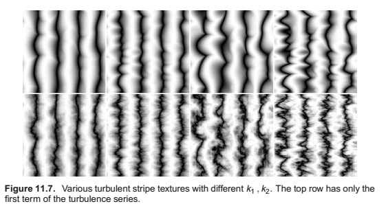
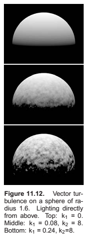
Turbulence

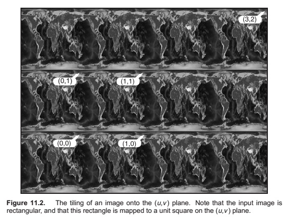
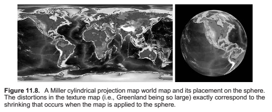
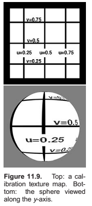
2D Texture Mapping
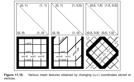
Texture Mapping for Rasterized Triangles
Perspective Correct Textures
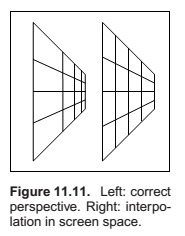
Corrected with interpolation in screen space,.
Compute bounds for \(x = x_i/h_i\) and \(y = y_i/h_i\)
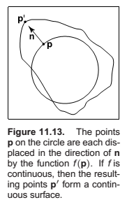
Bump Textures
Although we have only discussed changing reflectance using texture, you can also change the surface normal to give an illusion of fine-scale geometry on the surface. We can apply a bump map that perturbs the surface normal.
Environment Maps
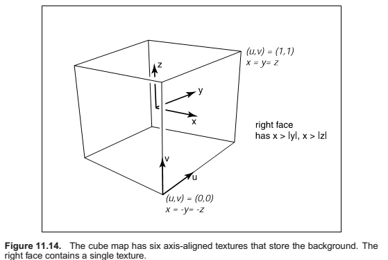
Often we would like to have a texture-mapped background and for objects to have specular reflections of that background. This can be accomplished using environment maps.
An environment map can be implemented as a background function that takes in a viewing direction \(\mathbf{b}\) and returns a RGB color from a texture map. There are many ways to store environment maps. For example, we can use a spherical table indexed by spherical coordinates. In this section, we will instead describe a cube-based table with six square texture maps, often called a cube map.
Shadow Maps
The basic observation to be made about a shadow map is that if we rendered the scene using the location of a light source as the eye, the visible surfaces would all be lit, and the hidden surfaces would all be in shadow. This can be used to determine whether a point being rasterized is in shadow.
Comments
comments powered by Disqus